Notes on When Models Manipulate Manifolds

Notes on When Models Manipulate Manifolds: The Geometry of a Counting Task (Gurnee et al., 2025), from Anthropic’s Transformer Circuits thread.

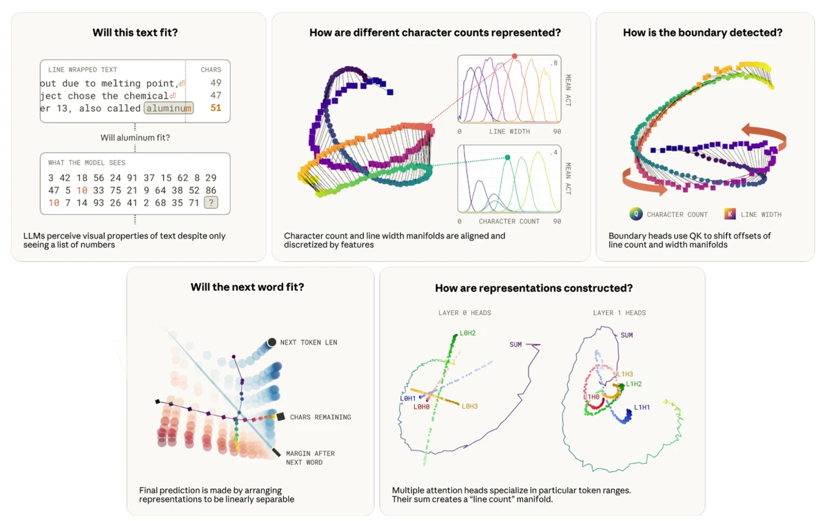
When a language model writes text wrapped to a fixed width, it has to break lines in the right places. That takes three numbers: how many characters are in the current line, how wide the lines in this document are, and how long the next word will be. None of them are in the input. Tokens arrive as integers with no character counts attached, and the line width is never stated anywhere — it has to be inferred from where the earlier lines happened to break.

Claude 3.5 Haiku does it anyway, for any width from 15 to 150 characters, usually correctly by the third line. The paper takes that mechanism apart and finds something closer to a perceptual system than to a semantic circuit: early layers that estimate position in the line, attention heads that compare that estimate against the inferred width, and a final decision that comes down to which side of a plane the answer falls on.

The count is carried by a curve

Take the first of those numbers. The line character count is how many characters have gone by since the last newline, including the current token — the model’s estimate of how far along the line it is. The obvious way to check whether Haiku tracks it is to fit a linear probe on the residual stream and see how the probe does. It does very well. After layer 1, linear regression recovers the count with an R² of 0.985.

That number means less than it looks like it means. A probe succeeding tells you the count can be recovered by a linear map. It does not tell you the model holds the count along a single direction, with small counts near the origin and large ones far from it, and the difference changes what the rest of the model can do with it.

What the model has instead is a family of features. Across a synthetic corpus of prose with its newlines stripped and reinserted at every width from 15 to 150 characters, binning each feature’s mean activation by character count turns up ten with smooth response profiles and large variance across counts. One fires at counts of roughly 35 to 55, the next at 45 to 65, and so on across the range (Fig. 1). Their receptive fields widen as the count grows, so a feature covering low counts spans a narrower band than one covering high counts, and the model resolves position more finely near the start of a line than deep into one.

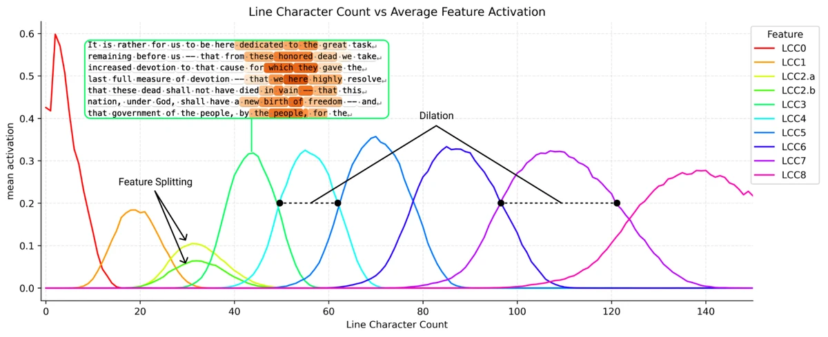
That arrangement shows up elsewhere. Curve detectors in vision models and place cells in a mouse running a linear track work the same way, carrying a continuous quantity across a set of discrete units each tuned to a band of values. The widening has a biological parallel too, since number representations in animal brains dilate the same way as the quantity grows. These are comparisons of coding geometry; they do not imply that the underlying mechanisms are shared.

Look at when those features are active and something shows up that the tuning curves hide individually. They rise and fall at an offset from each other, and for most values of the count, two are active at once. That is what you would expect if the ten features were sampling something continuous, each covering a stretch of it.

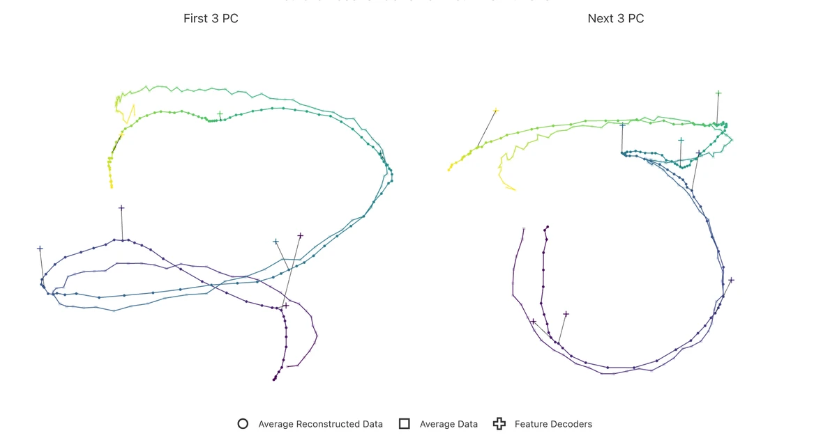
Averaging the residual stream at layer 2 for each of the 150 possible counts and running PCA on the result gives the thing being sampled. Six components carry 95% of the variance, and inside that subspace the 150 points trace one connected curve: a helix seen from the first three components, a more complicated twist from the next three. Reconstructing those same residual streams from only the ten features and projecting them into the same space lands almost on top of it (Fig. 2), with small kinks near each feature’s own direction, the way a spline bends toward its control points.

Testing the subspace

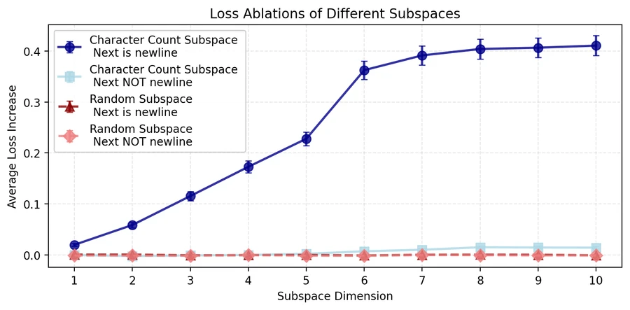
Is that curve doing any work, or is it an artifact of averaging? Two experiments say it is load-bearing. The first zeroes it out. Ablating the top few principal components of the per-count means at an early layer costs the model loss, and ablating a random subspace of the same size costs it much less. The gap appears only on tokens where the correct next token is a newline. Everywhere else the ablation barely registers, which is about what you would expect if the subspace is used for deciding where the line ends and for little else.

The damage also stops growing at the right place (Fig. 3). Removing more dimensions hurts more up to about six, and past six the curve flattens, which is an independent read on the same number the variance calculation gave.

That test needs a caveat the paper supplies itself. You cannot normally assume a subspace spanned by some features belongs to those features, because features share dimensions with each other, which is the packing pressure superposition describes. The argument for trusting it here is that the character-count subspace is densely active rather than sparse, since every token has a position, and densely active directions are poor candidates for sharing.

The second experiment changes the count instead of removing it. The paper’s running example is a prompt whose current line is 42 characters long and ends on the word called, where the word the model wants next is aluminum, ten more characters, which will not fit. To make the model believe it sits somewhere else in the line, subtract the average activation for the count it is actually at and add the average for a target count $c$:

Applied within six dimensions at three adjacent early layers, that shifts the model’s estimate of where it is and changes what it predicts, with six dimensions enough to push it either into or out of breaking the line.

Why the curve ripples

There is a fourth way to look at the count, and it exposes something the first three do not. Train 150 logistic probes, one for each possible count, and plot how each responds as the true count sweeps from 1 to 150. The result has the diagonal band you would expect, widening as the count grows, in line with the features. It also has faint bands running parallel on either side (Fig. 4). A probe tuned to count 42 falls off as the count moves away, then partly recovers, then falls off again.

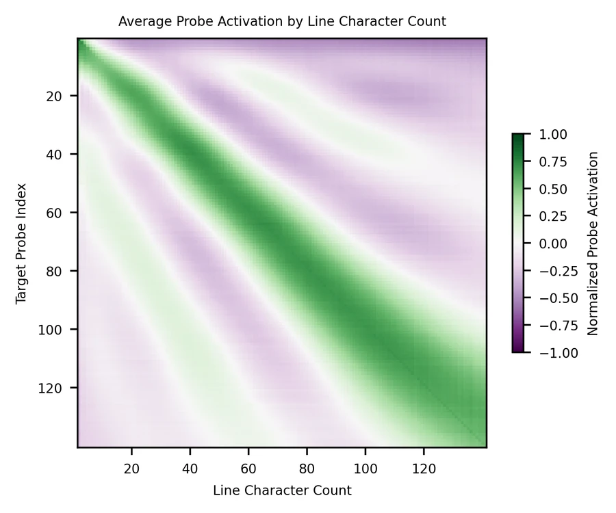
The paper calls this ringing, borrowing the signal-processing term for the oscillation that appears around a sharp edge, as in the Gibbs phenomenon. The same pattern shows up in the probe responses, in the cosine similarities between feature decoders, and in the per-count mean vectors. Neighboring features have positive similarity, features a moderate distance apart have negative similarity, and the sign keeps alternating as the distance grows.

The cause is a fact about geometry rather than anything specific to language models. Suppose you want 150 vectors arranged in a ring, each similar to its immediate neighbors and orthogonal to everything else. In 150 dimensions that is free. Squeeze the same arrangement into six and it cannot be satisfied, and the best available approximation, the one preserving as much of the original curvature as possible, buys accuracy near the diagonal by paying for it further out, in alternating bands of positive and negative similarity. The paper’s appendix makes this exact. The ideal similarity matrix is circulant, the discrete Fourier transform diagonalizes circulant matrices, so cutting down to six dimensions amounts to truncating a Fourier series, and truncated Fourier series ring. A simulation of 100 points on a six-dimensional sphere, pulled toward their near neighbors and pushed away from everything else, settles into the same ripples on its own.

That is worth restating in the vocabulary this thread usually uses. Ringing is interference. Superposition’s whole subject is what a model gives up when it packs more features into a space than that space has dimensions, and the cost it names is interference between features that should have been independent. Here the features are ordered along a scalar, so the interference lines up into visible stripes instead of scattering across unrelated concepts.

Comparing two curves

Knowing the position in the line is only useful alongside a second number: how wide the lines are. That is its own counting problem, solved the same way. Newline tokens carry their own family of counting features, tuned to the number of characters between one newline and the one before it, and those features trace their own curve.

So the model is holding two curves, one for how far along the line it is and one for how far it can go, and it needs to compare them. An attention score is a natural place to do that, because a score is already a comparison. For head $h$, the score from query position $q$ to key position $k$ is

The query and key projections only ever appear multiplied together, so they collapse into a single matrix sitting between the two residual streams. That matrix is a statement about which query directions match which key directions.

Give it two curves instead of two directions and it becomes a statement about how one curve sits relative to the other. What a boundary head does is rotate the character-count curve until it lines up with the line-width curve, offset by a little, so that count $i$ falls where width $i$ plus a small margin falls. The head then attends to the newline exactly when the current count is slightly short of the line width, which is the condition for the boundary being close. Before the twist the two families of probes sit apart; afterwards they run together (Fig. 5).

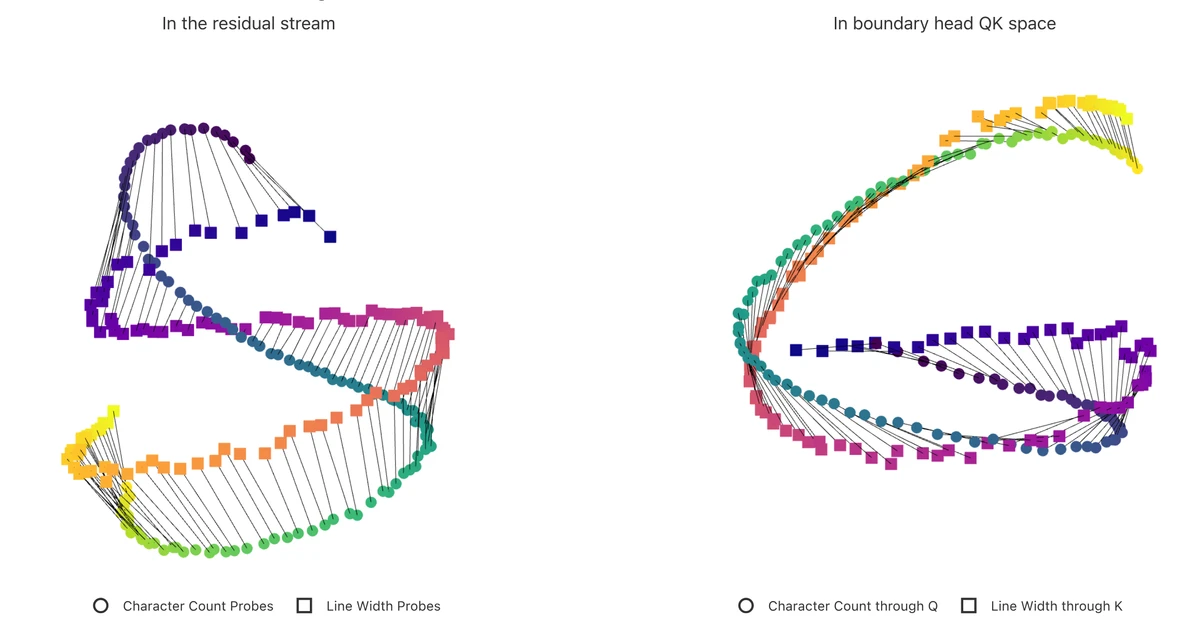
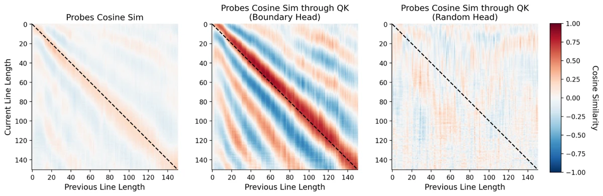
In the residual stream, the probe for count $i$ is most similar to the probe for width $i$, as you would hope, but the similarity is weak, about 0.25 at best. Pushed through a boundary head’s QK matrix, the same probes align almost perfectly, cosine similarity near 1, and the peak sits off the diagonal rather than on it. The same probes through a random head in the same layer show no structure at all (Fig. 6).

One boundary head is not enough, and the reason is a limit on what a single head can say. Its output is a weighted sum of what it attends to, passed through a fixed linear map, so the range of distinct values it can report is narrow. Five characters of headroom and seventeen characters of headroom come out of a single head looking much the same, which leaves too little resolution to decide whether a particular word will fit.

The model uses several, each twisting by a different offset, and their response curves tile the range between them. One varies most across the first ten characters of headroom, another across ten to twenty, a third across five to fifteen. Taken alone, each head’s output traces something close to a straight line. Added together they trace a curve, and positions along that curve are evenly spaced across the whole range that matters. The subspace holding that sum passes the same two tests the count subspace did: ablating it costs loss only where a newline was due, and substituting values into it moves the prediction.

That pattern is worth holding onto, because it recurs. A head’s output can only be as curved as its inputs already are, since all it does is take a weighted sum and apply a linear map. Curvature has to be assembled across several heads, each contributing a piece. The same constraint turns out to shape how the character count gets built in the first place.

Deciding to break

The third number is the length of the word the model is about to say, and it arrives late. The boundary detectors that fire about a third of the way through the model report how much room is left without knowing anything about the next word, so the two estimates have to be combined somewhere further on.

Around ninety percent of the way through, features appear that fire when the next word will overflow the line, alongside a matching set that fire when it will just barely fit. The first upweight the newline, the second push it down. Both families also do something less obvious, which is to suppress long tokens generally. If the model is wrong about which word comes next, whatever it says instead had better be short enough to fit.

The geometry underneath that decision is the tidiest result in the paper. Average the activations at that depth across every combination of characters-remaining and next-token-length, and the two quantities turn out to occupy near-orthogonal subspaces, each with only mild curvature. Their pairwise sums lay out on a grid, and the condition for breaking the line, that the next word is longer than the space left, becomes a plane cutting through that grid (Fig. 7). A hyperplane fit to the averages classifies real examples at an AUC of 0.91, which folds in both the classifier’s error and Haiku’s own uncertainty about what word is coming.

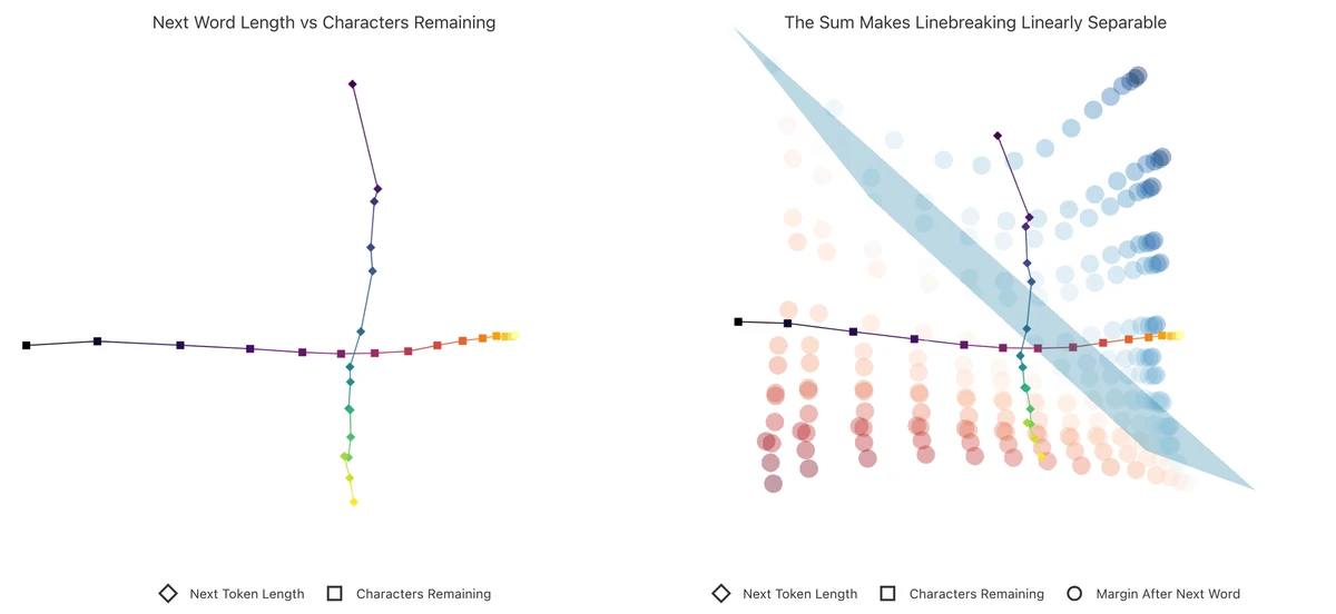
Worth naming the limit of the result. If the model were simply moving probability off every word that would overflow and onto the newline, then stripping the newlines out of the prompt should leave the rest of the distribution roughly intact. The two distributions differ substantially, so this is a decision about one candidate word rather than a filter applied across all of them.

Building the count

How does the count get built in the first place? This is the messiest part of the paper, and the part where the geometric account does least work on its own. Two simplifications make it tractable: attention heads move the count representation about four times as strongly as the MLPs do, and the count is already roughly readable after layer 0, so the analysis drops the MLPs and stays in the first two layers.

Each counting head there uses the previous newline as an attention sink. For the first few tokens of a line it attends almost entirely to that newline, then spreads across a window of recent tokens, and the OV circuit converts the pattern into an estimate. Parked on the newline, the line must be short, so the head writes toward low counts. Off the newline, the line must be at least as long as its window, so it writes toward the number of tokens in that window times an average token length of about four characters, adjusted by whether the tokens it sees run long or short.

Heads differ in how long they park and how wide their window is, so each covers a different stretch of the line, and each writes something close to a straight ray. The curve comes from their sum, the same assembly out of pieces the boundary heads needed. Five layer-0 heads recover the count with an R² of 0.93, and six more from layer 1 bring it to 0.97.

That is the whole mechanism (Fig. 8): perception in the first two layers, a comparison in the middle, and a linear decision near the output.

The line width is built much the same way, by a partly separate set of heads, since treating the previous newline as a sink needs adjusting when the current token is itself a newline. How the model aggregates one width from several previous lines is unresolved. It could be taking a maximum, or a decaying average of the recent ones, and the paper says it did not determine which.

What the geometry explains

The geometric account covers the parts of this task that are counting. Everything semantic stays in the feature view: the guess at the next word, the features that recognize what kind of continuation is wanted, the pathway that produces a plausible one. The paper is explicit that it relied on features alone for those, and the manifold story never reaches them.

Gaps remain inside the counting half too. The break decision is linearly separable in the geometry, but the analysis assumes the next word is a single token, and the authors say there must be structure they could not see that handles longer ones. Line-width aggregation is unresolved. So are the model’s handling of its own uncertainty about the count, documents whose width changes partway through, and special cases like a LaTeX \footnote{} or a markdown link.

Then there is the method’s own cost, which the paper states plainly. Parameterizing a manifold takes a lot of researcher time, and it works only when you already know the variable is continuous and can say what it is. Character count qualifies, and most of the concepts anyone would want to study do not.

The sharpest evidence about what the mechanism actually keys on comes from an adversarial test. Inserting the two-character string @@ into the prompt, without changing its length, disrupts the newline prediction. @@ opens a hunk in a git diff, a context where a line’s effective start is not the previous newline, and the counting heads have learned to treat it that way. In the altered prompt they split their attention between the previous newline and the @@ (Fig. 9).

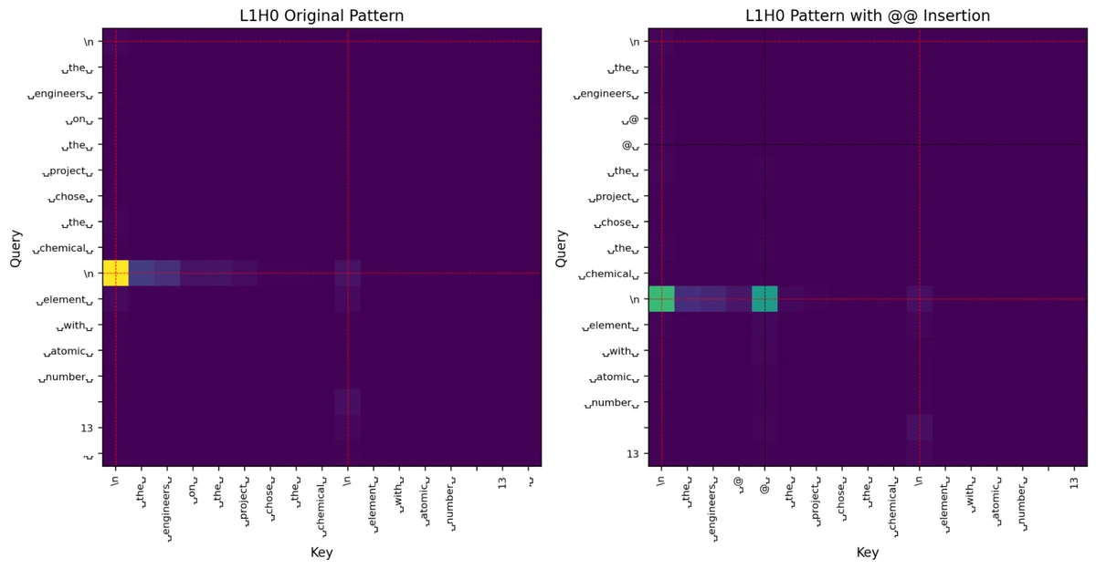
The effect is specific. Across 180 two-character insertions, most leave the newline as the top prediction and shift its probability only a little from a baseline of 0.79. The sequences that break it are almost all code delimiters, and how much a sequence disrupts the prediction tracks how far it pulls the counting heads off the newline.

The paper frames this as a visual illusion and compares it to Müller-Lyer, then hedges the comparison, which is the right call. The useful reading is narrower. What these heads detect is a learned cue about where a line begins, and that cue can fire on something that is not a line beginning.

The complexity tax

The paper opens its discussion with a methodological admission worth sitting with. The authors started by probing and patching, and it went badly. They had not yet separated line width from character count, so they were probing for a fused quantity the model does not represent, and they did not expect width to live only on newline tokens, so they were also looking in the wrong place. Their first probes were one-dimensional regressions besides, which is the wrong shape for a quantity that turns out to be a curve. Unsupervised features fixed all three problems. Even then, dozens of features looked vaguely like they were about newlines, and their differences only became legible once they were tested against a synthetic corpus with known ground truth.

So the dictionary earned its place. What follows is the complication. There are four descriptions of the character count in this paper and all of them are correct: ten sparse features, a six-dimensional subspace, a curve inside that subspace, and 150 probes. Each is good for a different job. Features found the thing to begin with. The subspace is what you intervene on. The manifold is what makes the boundary head describable as a rotation. The probes are what let you read that head’s weight matrices. The same duality runs through the computation itself, where the feature view sees a spray of virtual weights between feature pairs and the manifold view sees one twist.

The paper’s name for the gap between those descriptions is a complexity tax. Dictionary learning gives a true account of the computation, found automatically, which is a real result. Stopping there leaves you holding a description more complicated than the thing it describes. Recovering the geometry paid some of that back.

This is where the paper sits oddly in its own thread. The four papers before it are one continuous argument. Superposition says features are packed into too few dimensions, sparse autoencoders recover them, crosscoders extend the dictionary across layers, and attribution graphs assemble features into end-to-end traces. Each takes the last one’s output as its input, and the shared premise is that a large discrete dictionary is the right decomposition. This paper runs that whole stack, reports that it worked, and then says the result was more complicated than it needed to be.

It is also less of a departure than it looks. Ringing is interference, which superposition has been about since 2022. The boundary head is a QK circuit in the sense the 2021 framework paper defined, with an ordered family of features fed into it in place of two isolated directions. What changed is the vocabulary, and it changed because the features here happen to line up along a scalar, which makes the geometry visible. Read that way, the paper asks the superposition question again with better instruments.

Whether it is the last of its line is harder to say. The thread’s later work moves toward introspection, emotion concepts, and natural-language explanations of activations, which are different questions reached for with different tools. The call this paper makes is for methods that surface simpler structure automatically, since the geometry here was found by hand, and the authors describe what they did as an existence proof rather than a recipe.

Further material

• The paper’s interactive figures (opens in a new tab) include draggable versions of the counting manifolds and a simulation of the sphere-packing model that produces the ripples.
• The superposition notes cover the interference story that ringing turns out to be a special case of.
• The mathematical framework notes introduce the QK and OV split the boundary head is built from.
• The attention QK notes cover the attribution method that found this circuit before the geometry took over.
• Modell et al. (opens in a new tab) propose a formal notion of a feature manifold and report similar ripples and dilation in representations of colors, dates, and years.
• Michaud et al. (opens in a new tab) found linebreaking in fixed-width text among the top 400 behavioral “quanta” in a 70M-parameter Pythia model, which is why the paper treats it as a natural task rather than a contrived one.

References

These are notes on the work marked ★ — cite the original rather than this page.

1. Gurnee, W., Ameisen, E., Kauvar, I., Tarng, J., Pearce, A., Olah, C., & Batson, J. (2025). When Models Manipulate Manifolds: The Geometry of a Counting Task. Transformer Circuits Thread. https://transformer-circuits.pub/2025/linebreaks/index.html ★

Figures: Character-count, boundary-head, and illusion figures — from [1].