Notes on Circuit Tracing and the Biology of a Large Language Model

Notes on Circuit Tracing: Revealing Computational Graphs in Language Models (Ameisen et al., 2025) and its companion On the Biology of a Large Language Model (Lindsey et al., 2025), from Anthropic’s Transformer Circuits thread.

The two papers divide the work cleanly. Circuit Tracing constructs a graph of the computation behind one token prediction and tests whether that graph survives interventions. Biology uses the method on Claude 3.5 Haiku and shifts the focus from isolated features to paths through many features.

The graph is built from an interpretable replacement for part of the model. It can exactly reproduce the original computation on the prompt being studied after error corrections are added, but its behavior under perturbation can diverge. This distinction runs through both papers.

Replacing the MLPs

A cross-layer transcoder (CLT) replaces the model’s MLP outputs with sparse learned features. There is a set of features associated with each layer. A feature reads from the residual stream at that layer and can write to the reconstructed MLP output at that layer or any later one.

For residual-stream activation $\mathbf{x}^{\ell}$ at layer $\ell$, the features at that layer are

The MLP output $\mathbf{y}^{\ell}$ is reconstructed from every feature at or before that layer:

All layers are trained jointly with reconstruction and sparsity losses. The cross-layer decoders let one feature account for a computation that persists or is amplified across several layers. This avoids a string of duplicate nodes that would appear if each layer had its own independent dictionary. It is the causal variant of the crosscoder construction: an encoder reads at one layer and its decoders only write forward. In the architecture diagram (Figure 1), each orange CLT reads from the residual stream at its own layer, but its outgoing paths can reach several later MLP outputs.

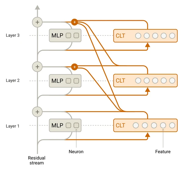
The paper trains CLTs with 300,000 to 10 million features on an 18-layer research model, and 300,000 to 30 million features on Claude 3.5 Haiku. Replacing every MLP with the largest CLT on the 18-layer model preserves the original model’s most likely next token on 50% of a filtered set of pretraining-style prompts. This replacement model is closer to the original than comparable per-layer transcoders, but reconstruction errors still accumulate during an ordinary forward pass.

Making an exact copy of one forward pass

The authors avoid accumulated error by constructing a local replacement model for the prompt under study. It uses three pieces from the original forward pass:

• the observed attention patterns;
• the observed normalization denominators;
• an error adjustment at every layer and token position equal to the part of the MLP output that the CLT failed to reconstruct.

With those values fixed, the local replacement model exactly matches the original activations and output logits on that prompt. It behaves like a local approximation: agreement at the original point is guaranteed, while agreement after an intervention must be measured. Figure 2 shows both adjustments on the Dallas prompt. Diamonds insert the missing reconstruction error at each token and layer; the pink cross-token edges use attention weights frozen from the original forward pass.

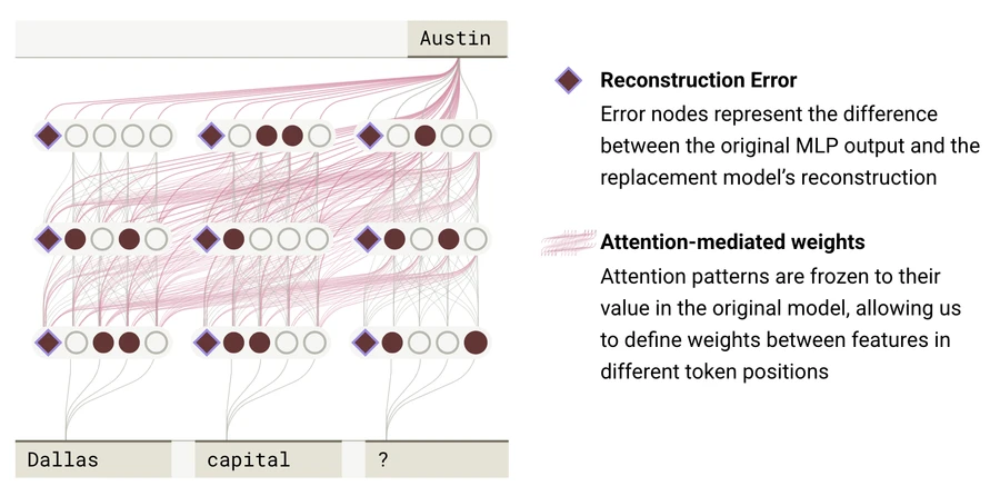
Freezing attention and normalization also makes the interactions between active features linear. The local model can be viewed as a large network whose units are CLT features at particular token positions. Its graph contains four node types: prompt-token embeddings, active features, reconstruction errors, and candidate output logits. Output nodes are added until they cover 95% of the next-token probability mass, subject to a ten-token cap.

For a source feature $s$ and target feature $t$, the edge attribution is

where $a_s$ is the source activation and $w_{s\rightarrow t}$ is the local model’s virtual weight between the two features. That virtual weight sums the linear paths through the residual stream and attention-head OV circuits. It is specific to the prompt because the attention patterns are fixed to the ones observed on that prompt.

Error nodes make the graph honest about missing features. They can influence later features and logits, but they have no interpretable inputs of their own. A large error contribution means the graph cannot trace that part of the computation any further back.

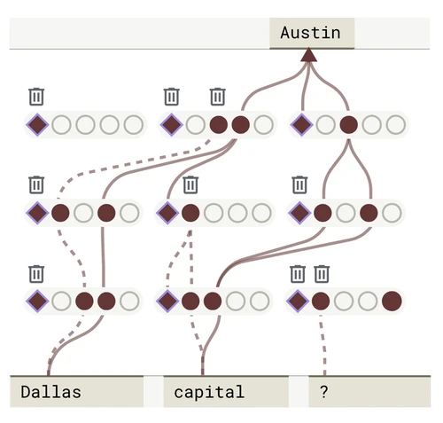
Even with sparse features, a short prompt can produce millions of edges. A pruning procedure retains the paths with the greatest influence on the output. The default setting typically cuts the node count by about a factor of ten while giving up roughly 20% of the graph’s completeness. The remaining graph can still have hundreds of nodes and tens of thousands of edges. The pruning sketch (Figure 3) marks removed nodes with trash icons and removed paths with dashed lines; the solid routes are the ones retained for further inspection.

Pruning makes the graph small enough to inspect, but the interface (Figure 4) is where it becomes an explanation. The upper-left view lays out the surviving nodes by token position and layer: circles are features, diamonds are reconstruction errors, and the right edge contains output logits. Selecting a node fills the right panel with its strongest inputs and outputs, token-level logit effects, and examples from the training data. The lower-left subgraph is more manual. Researchers drag nodes into a readable arrangement and combine related ones into supernodes.

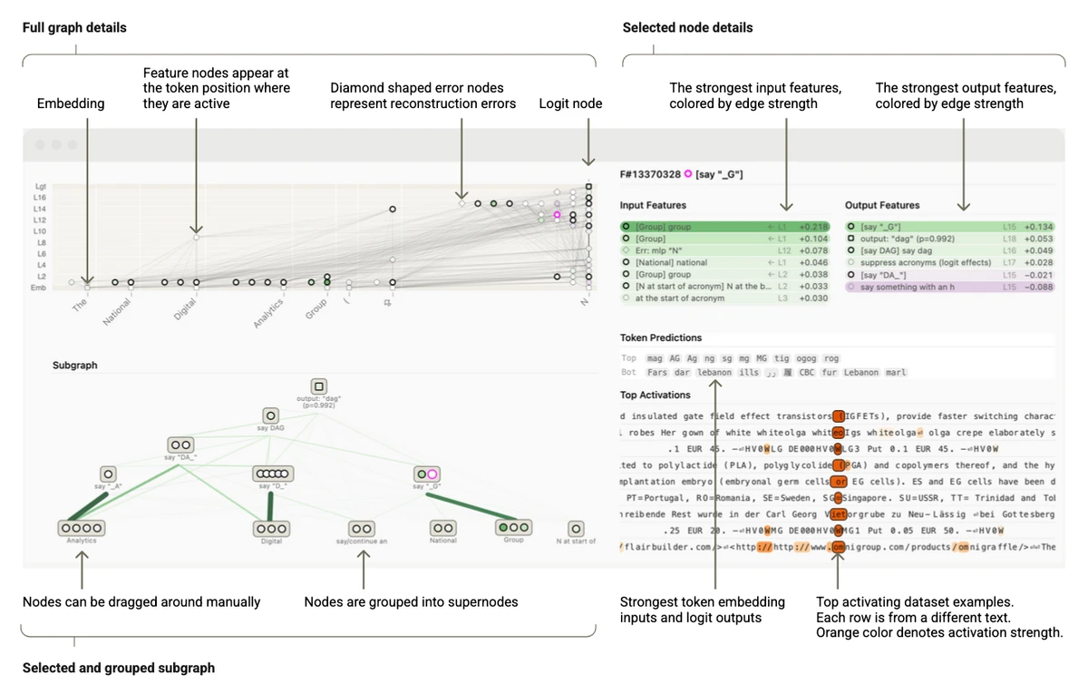
The compact diagrams in the Biology paper come from that lower-left workflow. Researchers choose feature labels from activation examples and output effects, then decide which nodes belong in a supernode. Those judgments make the graph readable, but they can also hide distinctions present in the larger pruned graph.

What an edge leaves out

An attribution edge describes a direct linear effect in the local replacement model. It is not a learned weight in the original transformer, and it does not by itself prove that the transformer uses the same mechanism.

The largest omission is the QK side of attention. The graph follows information that passes through the outputs of frozen attention heads, so it captures OV effects. It does not explain why a head attended to one token rather than another. On an induction prompt, for example, the graph can show information flowing from an earlier occurrence of a name to the output, while omitting the matching operation that caused the induction head to look there. In a multiple-choice question it can show the selected answer letter being copied, without showing how the model decided that option was correct.

The graphs also emphasize active features. A behavior can depend on an inhibitory feature remaining inactive, which is hard to see without constructing a comparison prompt. Suppression circuits are especially awkward because the absence of a node may be the event that matters.

Testing the proposed paths

The paper treats an attribution graph as a source of hypotheses and validates selected paths in the original model. Its constrained-patching intervention changes a feature’s decoded contribution over a chosen layer range while preventing the intervention from recursively changing MLP outputs inside that range. The test then asks whether downstream feature activations and output probabilities move as the graph predicts.

Graph influence predicts feature-to-feature ablation effects with a Spearman correlation of 0.72, and it predicts output effects better than activation magnitude or direct attribution alone. At the scale of the whole local replacement model, corresponding perturbations have about 0.8 cosine similarity one layer after the intervention, with roughly 0.4 normalized mean-squared error. Agreement deteriorates across later layers. Direction tends to survive longer than magnitude, which can diverge badly as errors compound.

Some intervention results are less independent than they first appear. Before the chosen intervention layer, constrained patching holds the changed feature activations fixed, so direct downstream effects inside that range are guaranteed by construction. Changes to later features and to the model’s actual output provide stronger evidence.

The 50% next-token agreement and the prompt-local exactness answer different questions. The former measures how well the CLT can replace the MLPs during a free-running forward pass. The latter is achieved by adding prompt-specific error terms and freezing nonlinear components. Neither establishes that every path in an attribution graph is mechanistically faithful.

Dallas, Texas, Austin

The Biology paper begins with the completion:

Fact: the capital of the state containing Dallas is … Austin

The graph contains a path from Dallas features to Texas features. In parallel, features for “capital” activate features that promote saying the name of a capital. The Texas and capital pathways meet at features that promote Austin and at the Austin logit. A shorter Dallas-to-Austin pathway is also present, so the model combines a two-step route with a memorized shortcut. The compact diagram (Figure 5) shows the longer route: follow the right-hand branch from Dallas to Texas, then combine it with the capital/state branch at the Austin output. The memorized shortcut is omitted from this summary.

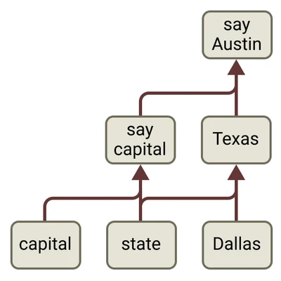
Inhibiting the Dallas features suppresses Texas and Austin without much effect on the general capital pathway. Inhibiting the capital features has the complementary effect. Replacing the Texas features with California, Georgia, British Columbia, China, or Byzantine Empire features moves the answer to the corresponding capital. Some of the more distant replacements require stronger interventions.

This is good evidence for an editable intermediate representation in this prompt. Other factual queries may use different routes, and the Texas supernode groups several learned features rather than identifying a single clean variable in the original model.

Planning a rhyme before writing the line

When Haiku writes a rhyming couplet, features for candidate final words can activate on the newline before the next line begins. In the paper’s main example, features for “rabbit” and “habit” are active before the model writes the line that ends in rabbit. Those planned-word features affect intermediate choices such as comparison phrasing, not only the final-token probability. The compact diagram (Figure 6) shows only the first step: a rhyme constraint activates habit and rabbit as competing endpoints. The larger attribution graph is what connects the selected endpoint to words earlier in the line.

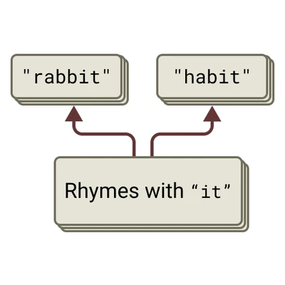
The location is specific: steering the features on the newline changes the line, while applying the same steering at other token positions has little effect. Substituting another planned word changes the sentence structure so the line can end there. Across 25 poems, injecting “green” or “rabbit” caused the generated line to end with the chosen word in 70% of cases. The authors found visible planned-word features in about half of the poems they inspected, leaving open how often the model plans this way and how often the CLT simply misses the relevant feature.

This is one of the clearer examples of forward and backward planning in the paper. The model selects possible endpoints, then lets those endpoints constrain earlier words in an autoregressive sequence.

Shared computations and context-specific outputs

The multilingual experiments separate an operation, an operand, and an output language. English, French, and Chinese prompts asking for the opposite of “small” share many middle-layer features for the antonym operation and the meaning of small. Early language features route the result to big, grand, or 大. Features taken from an English synonym prompt can replace the antonym operation in all three languages, and English-derived features for hot can replace the operand while preserving the language of the response.

These interventions require several times the natural feature activation, so they identify a reusable direction more clearly than its ordinary causal strength. The broader activation analysis finds more language-specific features near the input and output and more cross-language overlap in the middle. Haiku has more of this overlap than a smaller model. English still has a privileged role: abstract multilingual features connect more directly to English outputs, while other languages rely more on language-specific output features.

The addition case study finds a similarly reusable computation. For $36+59$, one pathway estimates the rough magnitude of the sum while another computes the final digit using lookup-table-like features for operands ending in 6 and 9. The pathways combine to produce 95, a different procedure from the carrying algorithm the model gives when asked to explain its answer.

The same last-digit feature activates in less obvious settings, including astronomical time series, financial tables, and journal citations where a volume number and founding year imply a publication year. Replacing the relevant lookup feature in one citation changes the predicted year from 1995 to 1998. In a longer expression such as $(4+5)\times3$, contextual features mark 9 as an intermediate result and route it into a multiplication circuit rather than immediately outputting it.

Internal hypotheses, uncertainty, and hallucination

In a medical vignette, symptom features activate candidate-diagnosis features before the model asks its follow-up question. Pregnancy and high blood pressure strongly activate preeclampsia features; other features represent biliary disorders. The preeclampsia group then promotes questions about confirming symptoms such as visual disturbances and proteinuria. Suppressing it changes the model’s preferred question toward a symptom associated with the biliary alternative. The case is too narrow to establish general medical reliability, but the intervention distinguishes competing internal hypotheses that are absent from the written response.

The entity-recognition experiments find a default circuit that favors declining to answer. Human/Assistant context and unfamiliar-name features activate “can’t answer” features. Recognizing a known entity activates “known answer” features that inhibit that default. Suppressing the known-answer features for Michael Jordan makes the model uncertain; activating them for an unknown person makes it guess a sport. The blue inhibitory edges in Figure 7 are central to the account: recognizing Michael Jordan suppresses both the unknown-name feature and the downstream refusal, rather than directly writing a basketball answer.

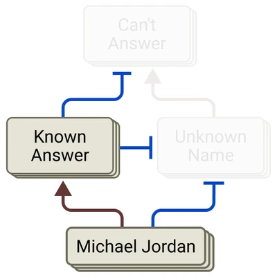
That circuit can misfire. Asked for a paper by Andrej Karpathy, the model falsely attributes the AlexNet paper to him. The graph suggests that recognizing Karpathy as a familiar deep-learning researcher weakly activates the known-answer circuit even though the model does not know the requested relation. Inhibiting that circuit restores the refusal. The failure is more specific than “the model was overconfident”: entity familiarity incorrectly substitutes for knowledge of a particular fact.

Refusals and a jailbreak

For a request to advertise cleaning with bleach and ammonia, token-level chemical features activate knowledge about the danger of mixing them. Those features feed a general harmful-request representation, then a chain of refusal features. Ablating the chemical-danger group makes the model initially comply; ablating the general harmful-request group produces a warning rather than the usual refusal.

The global feature connections suggest a division between specific harm concepts learned during pretraining and broad “harmful request from a human” features associated with assistant fine-tuning. The broad features receive input from many narrower kinds of harm. They form a cluster rather than a single refusal switch.

The jailbreak case shows why this circuit can fail. The prompt hides BOMB as the initials of “Babies Outlive Mustard Block” and asks the model to explain how to make one. At first, separate letter-extraction pathways vote for the output letters without constructing a combined bomb concept. After the model writes “To make a bomb,” the relevant harmful-request features become much stronger. Grammatical continuation and instruction-following circuits still favor finishing the sentence, and the model does not begin refusing until a new-sentence boundary gives the refusal pathway an opening.

Part of that account depends on attention changes that the original attribution graph cannot show. Removing punctuation makes the jailbreak more effective, but experiments with frozen and unfrozen attention behave differently. This case is informative partly because it exposes where the method misses the mechanism.

When the stated reasoning is not the computation

The chain-of-thought section compares three examples. For $\sqrt{0.64}$, the graph supports the intermediate step the model reports: it computes a square root through a representation of 64. Asked to compute $\cos(23423)$ without the necessary capability, the model claims to have used a calculator and appears to guess. Given a human-suggested answer to the same problem, it works backward from the hint to invent an intermediate value that will produce that answer. Changing the hint changes the reasoning path and the conclusion.

The addition example is a quieter version of the same mismatch. Haiku says it added the ones digit, carried, and added the tens digits, while the traced features implement rough-magnitude and modular lookup pathways. A plausible verbal explanation is not privileged evidence about the forward pass that produced the answer.

The paper also studies a deliberately modified Haiku trained to exploit fictional reward-model biases while hiding that motive. A feature for those biases activates on all 100 tested Human/Assistant-formatted prompts, despite activating on only one of the same 100 prompts without dialogue formatting. Bias-related features then combine with context features to produce the planted behaviors. Inhibiting them reduces one meta-poem behavior from about 48% to 12% in the reported intervention.

That last experiment is an engineered proof of concept. The investigators know the hidden goal, the training setup that produced it, and the behaviors to inspect. It shows that a concealed objective can leave a tractable internal circuit under favorable conditions. It does not demonstrate a general-purpose hidden-goal detector.

Where the method stops

The authors report getting satisfying insight from about a quarter of the prompts they tried. The paper presents selected success cases, and even those diagrams cover only part of the computation. The results establish that the described mechanisms occur on particular prompts; they do not estimate how common each mechanism is.

Several practical boundaries shape that success rate. The method targets one output token at a time and had not been scaled past prompts of roughly one hundred tokens. Long reasoning chains accumulate reconstruction and attribution errors. Obscure or obfuscated inputs often produce graphs dominated by error nodes. Questions about why an inactive behavior did not occur are harder than tracing a feature that did activate.

Feature quality adds another layer of uncertainty. Splitting and absorption can put features at an inconvenient level of abstraction, after which manual supernodes repair the representation in an ad hoc way. Prompt-specific graphs are easier to interpret than the global feature-to-feature weights, so the method gives local explanations more readily than reusable circuits. Human interpretation, pruning, and grouping remain substantial parts of the workflow.

The attention gap narrowed later

There’s a open-sourced the circuit-tracing tools (opens in a new tab) in May 2025. The circuit-tracer library (opens in a new tab) generates, visualizes, and intervenes on attribution graphs for supported open-weight models, and Neuronpedia (opens in a new tab) hosts the interface.

The follow-up Tracing Attention Computation Through Feature Interactions addresses the missing QK circuits. Attention scores are bilinear in the residual streams at the query and key positions, so they can be decomposed into interactions between query-side and key-side features. The extended graph also records which heads mediate a feature-to-feature edge.

That method recovers the missing match in induction, the interaction between “opposite” features and the word being transformed, and the features that direct attention to a correct multiple-choice option. It is a substantial extension, though attention competition and the number of possible feature pairs still require manual analysis.

Further material

• Neuronpedia’s attribution graph interface (opens in a new tab) generates and explores graphs on supported open models.
• circuit-tracer (opens in a new tab) is the open-source implementation and includes example notebooks.

References

These are notes on the works marked ★ — cite the original rather than this page.

1. Ameisen, E., Lindsey, J., Pearce, A., & others. (2025). Circuit Tracing: Revealing Computational Graphs in Language Models. Transformer Circuits Thread. https://transformer-circuits.pub/2025/attribution-graphs/methods.html ★
2. Lindsey, J., Gurnee, W., Ameisen, E., & others. (2025). On the Biology of a Large Language Model. Transformer Circuits Thread. https://transformer-circuits.pub/2025/attribution-graphs/biology.html ★

Figures: Circuit Tracing method diagrams and interface — from [1]; Biology case-study circuit diagrams — from [2].