Notes on Towards Monosemanticity and Scaling Monosemanticity

Notes on Towards Monosemanticity: Decomposing Language Models With Dictionary Learning (Bricken & others, 2023) and Scaling Monosemanticity: Extracting Interpretable Features from Claude 3 Sonnet (Templeton & others, 2024), from Anthropic’s Transformer Circuits thread.

Superposition leaves an awkward choice: analyze neurons that respond to several unrelated things, or try to recover a coordinate system closer to the features the model uses. These papers take the second route. They fit sparse autoencoders to a model’s activations, inspect the resulting directions, and test whether those directions are more coherent than the original neurons.

The autoencoder does not make the underlying model monosemantic. It is a post-training decomposition of its activations, and several decompositions can fit the same data. The question is whether sparsity is enough to make one of them useful.

Learning an overcomplete dictionary

Let $x$ be an activation vector from the model. A sparse autoencoder encodes it as a nonnegative feature vector $f(x)$ and reconstructs it from learned decoder directions:

The columns of $D$ are the candidate feature directions. There can be many more columns than dimensions in $x$, so the representation is overcomplete. The training loss balances reconstruction against an $L_1$ penalty on the feature activations:

The reconstruction term asks the dictionary to preserve the original activation. The sparsity term asks it to do so with only a few active features at a time. That second constraint is what makes an overcomplete dictionary recoverable rather than arbitrary.

The 2023 paper starts with the 512-dimensional MLP activations of a one-layer transformer. It trains dictionaries ranging from 512 to 131,072 features on eight billion activation vectors. Its main run has 4,096 features, eight times the dimensionality of the MLP. The setup diagram (Fig. 1) shows what is being expanded: the transformer stays fixed while the sparse autoencoder replaces 512 neuron coordinates with a larger set of candidate feature directions.

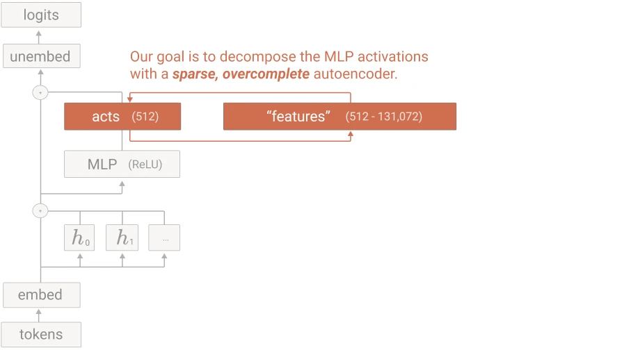
This setup follows directly from the superposition hypothesis. If a layer represents more sparse features than it has neurons, those features cannot each occupy a separate neuron. A sufficiently wide dictionary may still recover their directions from the pattern of activations.

Deciding whether a feature is good

There is no ground-truth list of the features in a language model, and the autoencoder’s loss is not an interpretability score. Low reconstruction error can coexist with polysemantic features. Heavy sparsity can produce a clean-looking dictionary that discards important behavior. Much of the first paper is therefore about how to evaluate a decomposition without pretending either proxy settles the question.

The authors inspect examples from across each feature’s activation range, not just its highest-activating tokens. This matters because an apparently clean feature can become muddled at low activations. They compare the examples with computational proxies, ask human raters to describe blinded samples, and use language models to predict activations and output effects from feature descriptions. Across these tests, the learned features score as more interpretable than individual neurons. In the automated output-weight test, feature descriptions identify tokens with large positive output weights 74% of the time, compared with 58% for neuron descriptions and 50% at chance.

The main 4,096-feature run is not uniformly clean. Of its learned features, 168 never activate and another 292 activate so rarely that the paper excludes them from much of the analysis. Among the remaining features, interpretability is strongest at high activation values and less reliable near zero.

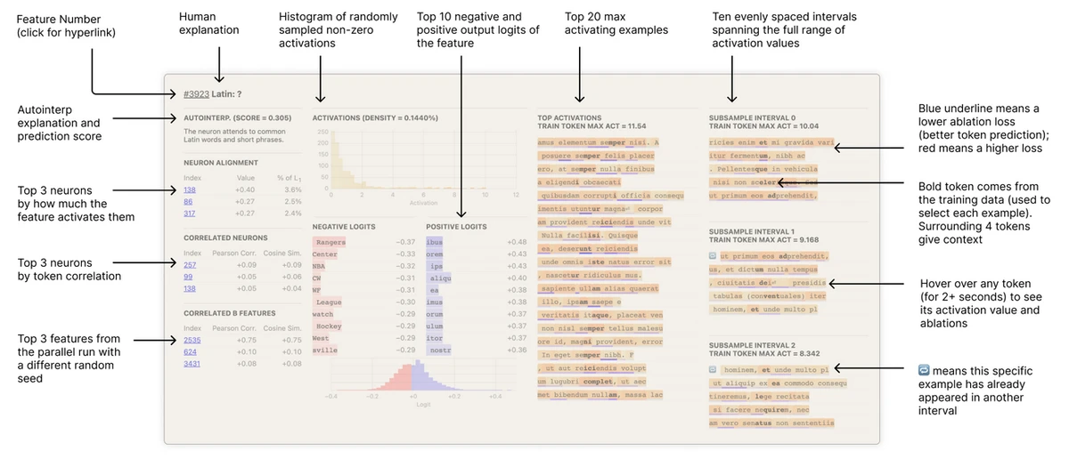
The feature interface below (Fig. 2) is designed around that problem. The histogram shows how frequently different activation strengths occur, while the logit columns show which outputs the feature promotes or suppresses. On the right, the maximum-activating texts sit beside samples drawn across the full activation range. Those range samples are where a clean label often starts to break down. The links on the left compare the feature with individual neurons and with features learned in another run.

The Arabic-script feature

The paper develops four hand-picked examples in detail: features for Arabic script, DNA sequences, base64 text, and Hebrew script. These are unusually legible cases, not a random sample, but they show what a serious claim of monosemanticity requires.

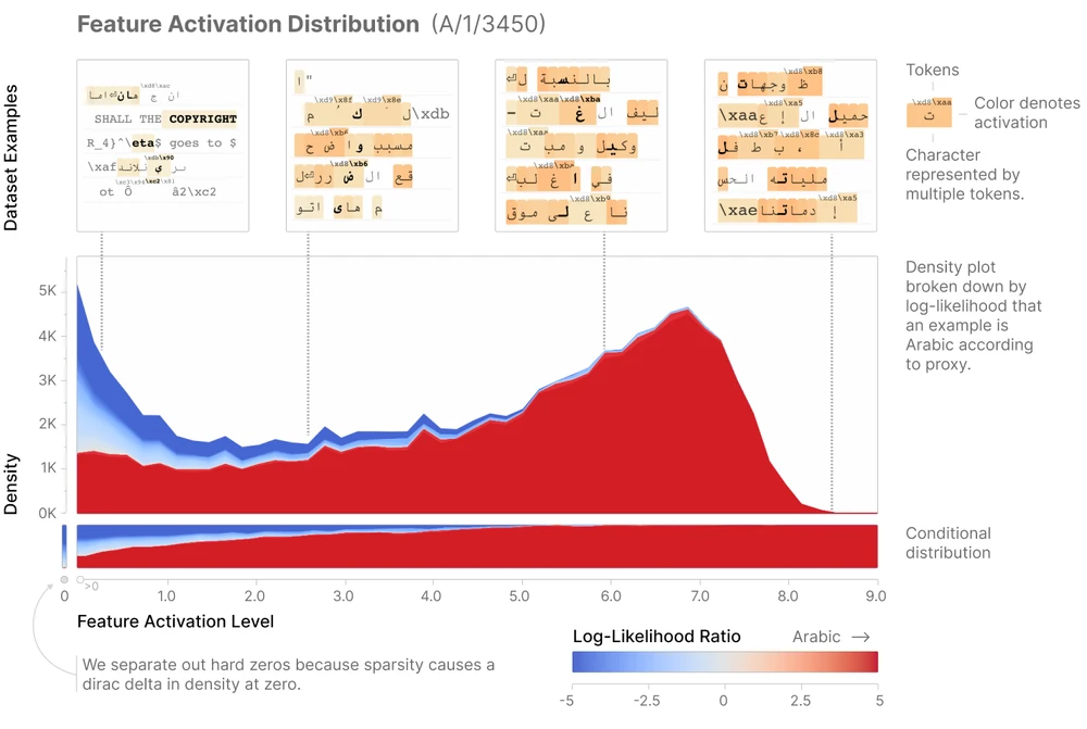
For the Arabic feature, the authors construct a proxy that estimates how likely each token is to be Arabic script. Arabic accounts for 0.13% of the data but 81% of the tokens on which the feature is active. Above an activation of 5, the proportion rises to 98%. The residual low-activation cases are important: the feature is highly specific when strongly active, but not literally perfect across its full range. In the activation plot (Fig. 3), this appears as an almost pure right tail and a more mixed cluster near zero.

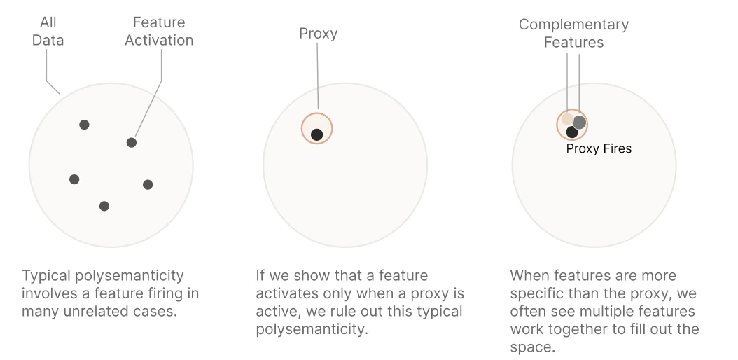
Specificity is only half of the test. A feature might fire exclusively on Arabic while covering only a narrow corner of Arabic text. The paper also measures sensitivity and looks for nearby features that cover examples this one misses. That comparison turns a plausible label into a claim about which part of the data distribution the direction represents. The proxy diagram (Fig. 4) separates the two failure modes: unrelated feature activations count against specificity, while proxy-positive examples missed by the feature count against sensitivity and may reveal narrower neighboring features.

The feature also has effects consistent with its interpretation. Its decoder direction favors Arabic tokens in the output logits, and forcing it active makes the model produce Arabic text. The corresponding intervention on the base64 feature produces base64-like output. These experiments show that the directions are not labels attached after the fact: changing them can change the model in the expected direction.

They do not show that one direction is solely responsible for a behavior. Intervening through an autoencoder changes a reconstructed activation, and large interventions can move it away from states encountered in ordinary inference. Causal usefulness is a stronger result than correlation, but it is not a complete circuit explanation.

The selected features also fail to line up with any single neuron. Some never appear among the top examples for any neuron, despite being clear in the learned dictionary. Training autoencoders on two separately trained one-layer models recovers more similar feature directions than comparing their neurons directly. That is evidence that the dictionaries track recurring structure, though not that every run recovers a unique set of features.

Reconstruction gives a separate measure of coverage. Substituting the main autoencoder’s reconstruction for the original MLP activation preserves 79% of the improvement in language-model loss contributed by the MLP; the 131,072-feature run preserves 94.5%. Those numbers measure behavioral fidelity under one ablation comparison. They should not be read as the percentage of the model that has been interpreted.

Dictionary width changes the grain

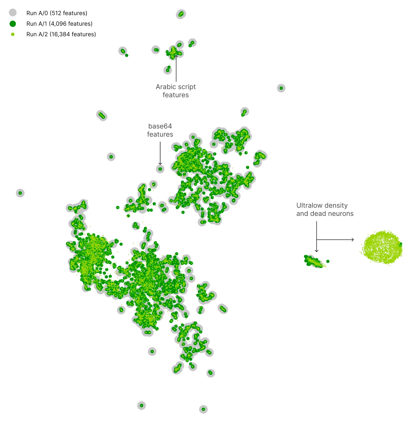
As the dictionary gets wider, coarse features often divide into more specific ones. The base64 region is a clean example: a small dictionary contains a broad base64 feature, while larger dictionaries separate token patterns and contexts that the smaller run groups together. The UMAP compares whole dictionaries at once. Nearby points indicate similar decoder directions across widths; the isolated region of dead and very rare features is a warning that proximity alone is not evidence of a meaningful concept.

The sketch below (Fig. 6) is a model of what one local neighborhood in that projection can mean. A direction learned by the narrow dictionary may correspond to several more specific directions once the dictionary has enough capacity to separate them.

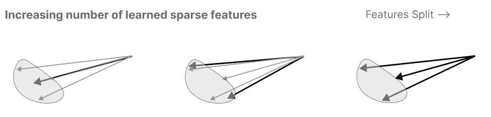
“Splitting” is useful shorthand, but the relationships do not form a neat tree. Features can split, merge, or be rearranged between runs. Dictionary width is partly a resolution setting: a feature that looks polysemantic at one width may be a compromise over a family of related features, while a very wide dictionary may devote directions to rare token-level distinctions.

This makes talk of the model’s features slippery. The geometry appears to contain stable regions, but the individual units returned by an autoencoder depend on its width, sparsity penalty, training data, and optimization. A learned feature is best treated as a candidate coordinate in a useful decomposition, not an indivisible object recovered from the model.

Moving from one layer to Claude 3 Sonnet

Scaling Monosemanticity applies the same basic method to the middle-layer residual stream of Claude 3 Sonnet. This is a different target from the MLP activations in the first paper. The residual stream is a shared communication channel between components, and using one layer keeps the extraction problem tractable, but it also gives only one cross-section of the model’s computation.

The paper trains autoencoders with roughly one million, four million, and 34 million features. Fewer than 300 features are active on an average token, and the reconstructions explain at least 65% of the activation variance. Scale also makes optimization waste visible: about 2% of the one-million-feature dictionary is dead, rising to 35% for four million and 65% for 34 million.

Sweeps over dictionary width and training duration produce approximate scaling laws for the autoencoder’s reconstruction-plus-sparsity loss. The compute-optimal dictionary gets wider as the training budget grows, while the optimal learning rate falls. These laws help allocate SAE training compute. They do not establish that a lower SAE loss produces a more interpretable dictionary, a distinction the paper flags as an unresolved evaluation problem.

Many of the resulting features are more abstract than the script and encoding features in the one-layer model. A Golden Gate Bridge feature activates for references to the bridge in several languages and in images, even though the autoencoder was trained on text activations. A code-error feature responds to invalid operations and mistakes in Python, C, and Scheme without responding to ordinary English typos. Another feature recognizes addition performed through function composition rather than matching a particular piece of syntax.

The features are again difficult to reduce to neurons: for 82% of a sampled set, the highest correlation with any neuron in any preceding layer is at most 0.3. Automated evaluations also rate random SAE features as more interpretable and specific than neurons. These results extend the central observation of the first paper, while relying more heavily on automated judgments because millions of features cannot be checked by hand.

Feature steering supplies vivid causal examples. Increasing the Golden Gate Bridge feature makes the model mention the bridge and, at a ten-times-maximum clamp, claim to be the bridge. Steering the code-error and addition features also changes the corresponding outputs. The extreme Golden Gate intervention is useful for identifying the direction’s effect, but it says little about the feature’s normal causal importance; at large enough values, feature steering often makes the model repetitive or incoherent.

The paper also finds features related to sycophancy, deception, secrecy, unsafe code, and other safety-relevant topics. Their presence shows that these concepts are represented in a form the autoencoder can expose. It does not distinguish between discussing a behavior, recognizing it in someone else, being capable of it, and pursuing it.

What scaling did not settle

The 34-million-feature dictionary is still incomplete. As a concrete test, the authors find dedicated features for only about 60% of London boroughs even though Claude can list all of them. Rarer concepts tend to require wider dictionaries, and extrapolating that relationship suggests that comprehensive coverage could need dictionaries far larger than the model itself. A missing dedicated feature also does not mean a concept is absent from the model: it may be assembled from several broader features.

There are structural limits as well. Features can be spread across layers, so an autoencoder at one residual-stream location may merge computations that become distinct elsewhere. The $L_1$ penalty shrinks feature activations and introduces reconstruction bias. Automated descriptions have no reliable ground truth, and reconstruction loss, sparsity, and interpretability can disagree. Extracting directions also leaves the attention patterns and upstream circuits that create them unexplained.

The scaling result is therefore narrower than “millions of monosemantic concepts were found.” It shows that sparse dictionary learning continues to produce many coherent, causally usable directions in a much larger model. It does not provide a canonical inventory of the model’s concepts or a complete account of how those concepts are computed.

What later work added

The method became easier to test outside Anthropic after DeepMind released Gemma Scope (opens in a new tab), a collection of more than 400 open sparse autoencoders across Gemma 2’s layers and sublayers. That infrastructure made comparison easier, but it also exposed disagreements between evaluation criteria.

SAEBench (opens in a new tab) evaluates autoencoders on seven metrics. Its rankings show that a good sparsity-fidelity tradeoff does not reliably predict performance on downstream or disentanglement tests. One reason is feature absorption (opens in a new tab): a seemingly general feature may fail to activate on some valid examples because a more specific feature has taken them over. Simply changing dictionary width or sparsity does not consistently remove the problem.

DeepMind’s mechanistic-interpretability team later reported negative results on downstream tasks (opens in a new tab). No single experiment rules SAEs out, but the team did not find a convincing advantage over simpler baselines for the tasks it tested and chose to deprioritize the approach. A subsequent position paper makes a useful distinction: use SAEs to discover unknown concepts, not to act on known concepts (opens in a new tab). If the target concept is already specified, supervised probes can be simpler and more reliable. The distinctive promise of an SAE is unsupervised discovery: surfacing candidate structure that an investigator did not know to look for.

That is a more modest role than a complete reverse-engineering method, but it fits the strongest evidence in the original papers. Sparse autoencoders are good at proposing directions worth investigating. The work of checking what a direction means, when it fails, and how it participates in a circuit remains.

Further material

• Neuronpedia (opens in a new tab) provides interfaces for browsing features from open models.
• SAELens (opens in a new tab) is a library for training and analyzing sparse autoencoders.
• ARENA’s sparse-autoencoder exercises (opens in a new tab) walk through training a small SAE and inspecting its features.

References

These are notes on the works marked ★ — cite the original rather than this page.

1. Bricken, T., & others. (2023). Towards Monosemanticity: Decomposing Language Models With Dictionary Learning. Transformer Circuits Thread. https://transformer-circuits.pub/2023/monosemantic-features/index.html ★
2. Templeton, A., & others. (2024). Scaling Monosemanticity: Extracting Interpretable Features from Claude 3 Sonnet. Transformer Circuits Thread. https://transformer-circuits.pub/2024/scaling-monosemanticity/index.html ★