GPU Simulation: Warp Scheduling & Compute/Tensor Cores

Introduction: Seeing Inside the GPU

Profiling tools like NSight Compute give you numbers: throughput, latency, stall reasons. But they don’t let you reach inside the scheduler and change how it works. For that, you need a simulator.

Projects 3 and 4 of Georgia Tech’s CS 8803: GPU Hardware and Software put you inside a stripped-down GPU simulator called Macsim. You’re not running CUDA kernels. You’re implementing the hardware mechanisms that make CUDA kernels run. That shift in perspective is, in my view, the most intellectually interesting part of the course.

Project 3 asks: how should a GPU decide which warp to run each cycle? Project 4 asks: once you include the latency of compute instructions (not just memory), how does the picture change, and how do tensor cores fit in?

Trace-Driven GPU Simulation

Before getting into warp scheduling specifics, it’s worth understanding what kind of simulator Macsim is and why trace-driven simulation exists.

Why Simulate at All?

When you profile a real GPU program, you get aggregate statistics: average stall cycles, cache miss rate, achieved occupancy. You can’t easily answer questions like “what if the warp scheduler used a different policy?” or “what if the L1 cache were twice as large?” Answering those questions requires either expensive hardware modifications or a simulator.

Simulators are slower than real hardware, often by orders of magnitude, but they give you complete observability and controllability. You can read any internal state at any cycle, inject faults, or swap out entire subsystems. Architects use them constantly when designing new hardware.

Trace-Driven vs. Execution-Driven

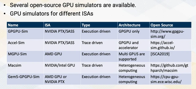
There are three broad approaches to GPU simulation.

Execution-driven simulation re-executes the actual program inside the simulator. It’s accurate but slow because every instruction has to go through the simulated pipeline.

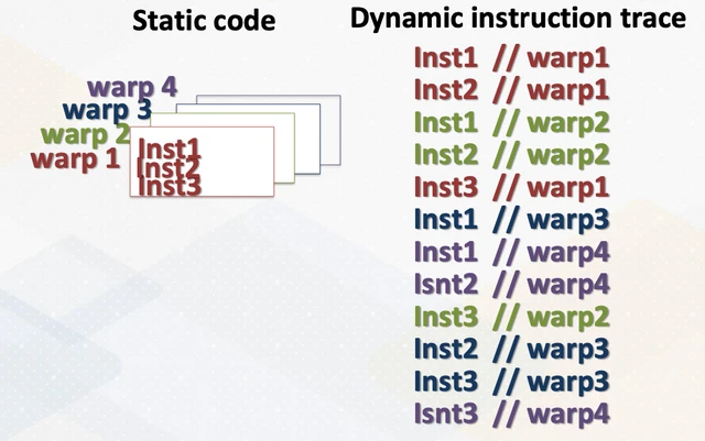
Trace-driven simulation pre-records a trace of all instructions that a program executes on real hardware, then replays that trace through the simulator. The trace capture happens once (Macsim uses NVBit for this), and then simulation is fast because the simulator just reads the trace rather than re-evaluating the program logic.

Sampling / interval simulation models only selected windows of execution (or aggregates behavior over intervals) rather than replaying every instruction. It’s dramatically faster for design-space exploration, but less precise for fine-grained microarchitectural effects.

The tradeoff: trace-driven simulation can’t model data-dependent control flow changes that would arise from different hardware behavior. But for studying things like cache behavior and scheduling policies (where the instruction stream itself doesn’t change), it’s a practical and widely-used methodology. That’s why this project used a trace-driven, cycle-level setup: enough fidelity to reason about scheduler/cache effects, without execution-driven runtimes.

The Macsim Architecture

Macsim is a stripped-down trace-driven GPU simulator. Its structure maps directly to real GPU hardware:

• A trace reader (trace.h) that parses NVBit-generated instruction traces
• Multiple GPU cores (core.cpp), each with its own dispatch queue of active warps and a suspended queue for warps waiting on memory
• An L1 cache per core and a shared L2 cache (cache.cpp)
• A simple fixed-latency memory (ram.cpp)

Each core runs one warp per cycle. When a warp executes a load or store, it moves from the dispatch queue to the suspended queue until the memory response arrives. When all cores exhaust all warps, simulation ends.

A cycle in Macsim looks like this:

1. Check for returned memory responses; move corresponding warps from suspended → dispatch queue
2. Move the previously executing warp back to the dispatch queue
3. If both queues are empty, request a new batch of warps
4. Schedule one warp from the dispatch queue using the current policy
5. Execute one instruction for the scheduled warp

Step 4 is where Projects 3 and 4 live.

Warp Scheduling: The Dispatcher’s Dilemma

Why Scheduling Policy Matters

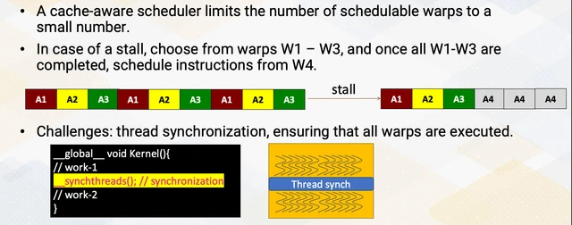
A GPU core has many warp contexts loaded simultaneously. The point of this design is latency hiding: when one warp stalls waiting for memory (hundreds of cycles), the core switches to another warp and keeps the functional units busy. This is the GPU’s alternative to the CPU’s approach of deep out-of-order execution and large caches.

But latency hiding and cache performance are in tension. Here’s the conflict:

• Maximum latency hiding wants as many warps in flight as possible, so when any one warp stalls, others are always ready. This argues for Round Robin scheduling: cycle through every warp evenly.
• Cache efficiency wants data to stay warm in the cache. If you interleave too many warps, the cache gets thrashed: each warp brings in its working set, evicts the previous warp’s data, and then when the previous warp resumes it gets cache misses all over again.

The right scheduling policy depends on the workload. Cache-intensive applications need to trade some latency hiding for better locality. This is the core tension Project 3 explores.

Two-Level Warp Scheduling

Macsim implements a two-level scheduling scheme that mirrors how real GPU hardware works.

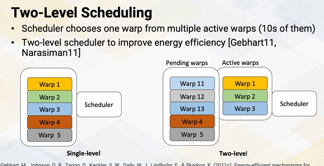
The outer level manages which warps are eligible to be scheduled (the dispatch queue). The inner level picks among the eligible warps each cycle. The scheduling algorithms you implement operate at the inner level.

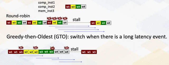
Round Robin: The Baseline

Round Robin (RR) is the simplest possible policy: each cycle, pick the next warp in a circular queue. It’s fair, every active warp gets equal time, and it maximizes latency hiding because you always switch to a different warp after each instruction.

The cost shows up in the cache. RR cycles through all warps rapidly, which means each warp’s working set is competing with every other warp’s working set. On a workload with temporal locality within each warp (the same address accessed multiple instructions apart within the same warp), RR destroys that locality.

Greedy Then Oldest (GTO)

GTO is a more sophisticated policy with a simple intuition: if the current warp is still runnable, keep running it. Only switch away if it stalls.

if (last_scheduled_warp is still in dispatch queue):
    schedule last_scheduled_warp
else:
    schedule the oldest warp in the dispatch queue

“Oldest” is defined by a timestamp: the warp that has been waiting the longest without being scheduled. This prevents starvation.

GTO reduces stall cycles because it extracts more work from each warp before switching. If warp A’s instructions have no memory stalls, GTO will run A through its entire ready sequence before touching warp B, which is more efficient than interleaving them. And when A does stall, switching to the oldest waiting warp means you’re picking the warp that’s been waiting longest, which in practice tends to be the one whose memory response has (or soon will have) arrived.

The grading metric for Task 1 was NUM_STALL_CYCLES. GTO reduces stalls compared to RR in many workloads, which is why it remains a common research baseline and often performs strongly in simulator studies.

Simplified Cache-Conscious Wavefront Scheduling (CCWS)

GTO improves stall cycles but doesn’t directly address cache thrashing. CCWS takes a different angle: dynamically limit how many warps are allowed to compete for the cache.

The insight from the CCWS paper (Rogers, O’Connor, Aamodt, MICRO 2012): if a warp’s data gets evicted from cache by other warps before that warp gets a chance to reuse it, those evictions are wasted bandwidth. A “victim tag array” (VTA) per warp can detect this: it stores the tags of lines evicted from L1. When a warp later misses in L1 and hits in its own VTA, that’s evidence of lost locality, meaning the eviction was premature and the warp would have reused that data if it had been given more cache.

Each warp maintains a Lost Locality Score (LLS) that quantifies how much locality it has lost. The score is computed as:

LLS = (VTA_Hits_Total × K_Throttle × Cum_LLS_Cutoff) / Num_Instr

where Cum_LLS_Cutoff = Num_Active_Warps × Base_Locality_Score.

In this project context, this exact score/cutoff form comes from the course’s simplified CCWS model and grading harness rather than a claim about production GPU firmware policy.

Each cycle, warp LLS scores decay by 1 (down to a minimum floor), so the throttling is transient. If the locality situation improves, more warps are re-admitted. Warps are sorted by LLS in descending order, and the top warps whose cumulative scores fall within the cutoff form the schedulable set. Round Robin then applies within that set.

The grading metric for Task 2 was MISSES_PER_1000_INSTR. CCWS improves cache miss rate by throttling the warp count just enough to let each warp’s working set fit comfortably in the cache.

Design Questions This Raised

Working through the CCWS implementation, several architectural questions stayed open:

• How do you tune K_Throttle? A higher value means more aggressive throttling, with fewer warps allowed. Too aggressive and you sacrifice latency hiding unnecessarily. Too conservative and you don’t help the cache. The right value is workload-dependent, which raises the question of whether a self-tuning version could be built.
• What happens at the boundary? When the LLS scores change enough that a warp is admitted or expelled from the schedulable set, there can be abrupt shifts in behavior. How do real implementations smooth this transition?
• CCWS only helps if there’s actual intra-warp temporal locality. For a workload with purely streaming access patterns (no data reuse), reducing the warp count hurts latency hiding with no cache benefit. How should the scheduler detect this?

Compute and Tensor Core Modeling (P4)

Project 3’s Macsim only simulates load/store instructions, while compute instructions (adds, multiplies, FMAs) are ignored. This is a simplification that makes sense when you’re studying cache behavior, but it misses a large part of what happens on a real GPU.

Project 4 extends the simulator to model compute instruction latency. Once compute latency matters, scheduling behavior changes significantly.

The Execution Buffer

In a real GPU pipeline, an instruction doesn’t complete instantaneously. A floating-point multiply has some number of pipeline stages. While that instruction is in flight, the registers it will write are not yet valid, so a subsequent instruction that reads those registers must wait.

A central addition in Project 4 is an execution buffer: a per-core data structure that tracks in-flight compute instructions. Each entry stores:

• The instruction being executed
• The cycle at which it will complete (i.e., when its output register becomes valid)

Each cycle, the simulator:

1. Checks the buffer for entries whose completion timestamp has passed, and removes them (the register is now valid)
2. When scheduling a new compute instruction, adds it to the buffer with completion_cycle = current_cycle + latency
3. If the buffer is full, stalls the warp, because it can’t issue another compute instruction until a slot opens up

This is the mechanism that makes compute throughput finite. Without the buffer, every instruction would complete in one cycle, regardless of latency.

// Conceptual execution buffer management, not project-specific code
struct ExecEntry {
    Instruction* instr;
    uint64_t     completion_cycle;
};

vector<ExecEntry> exec_buffer;

// Each cycle: retire completed instructions
for (auto it = exec_buffer.begin(); it != exec_buffer.end(); ) {
    if (current_cycle >= it->completion_cycle) {
        it = exec_buffer.erase(it);
    } else {
        ++it;
    }
}

// Issue new compute instruction
if (exec_buffer.size() < EXEC_WIDTH) {
    exec_buffer.push_back({ instr, current_cycle + instr->latency });
} else {
    stall_warp();
}

The grading metric for Task 1 was NUM_CYCLES, the total cycle count to complete the gemm_float trace. Getting this right means correctly modeling when warps stall due to a full execution buffer.

Scoreboarding and Register Dependencies

Once instructions have multi-cycle latency, you have to think about register hazards. The classic case is a read-after-write (RAW) dependency: instruction B reads a register that instruction A is still writing. If B executes before A completes, B reads stale data.

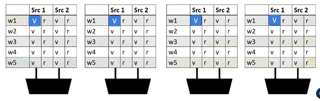
The standard hardware solution is scoreboarding: a register file annotation that marks each register as either available or pending (being written by an in-flight instruction). Before an instruction issues, the scheduler checks that all its source registers are available. If any are pending, the warp stalls until they’re cleared.

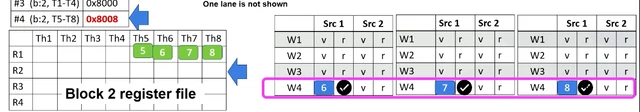
In Project 4’s Round Robin scheduler, this means a warp should be skipped when the warp’s next instruction has a source register that’s still in-flight. The scheduler must iterate through warps to find one whose instruction is dependency-free, rather than always picking the next warp in order.

Extending to Tensor Cores

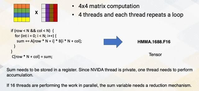
Task 2 of Project 4 extends the compute core model to simulate tensor core behavior. This required understanding what makes tensor cores fundamentally different from regular CUDA cores.

Two differences from regular CUDA cores matter most:

Execution width: A tensor core processes multiple operations simultaneously per cycle, so execution width is greater than 1. In the project, the configured width is 8: up to 8 tensor instructions can be in the execution buffer at once, compared to 1 for a regular compute instruction. This reflects how tensor cores are physically wider, with more multiplier arrays.

Latency: Tensor instructions (HMMA, half-precision matrix multiply-accumulate) have much higher latency than regular FP32 instructions. The configured latency is 64 cycles, vs. a default of 1 cycle for other compute instructions. This reflects the deep pipeline in a real tensor core.

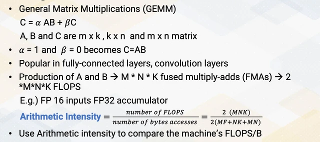
Instruction count: Because each tensor instruction computes more work per instruction (a whole tile MMA), the total instruction count for a GEMM done with tensor cores (gemm_half) is much lower than the same GEMM done with scalar FFMA instructions (gemm_float). The total work is the same, but the instruction-level “packaging” is different.

In code, detecting a tensor instruction amounts to checking whether the opcode starts with H* (HMMA opcodes). If yes: use width=8 and latency=64. If no: regular compute core behavior.

Sensitivity Analysis

The report for Project 4 required plotting how NUM_STALL_CYCLES and NUM_CYCLES varied as you swept tensor latency (32–128) and execution width (2–16). In these sweeps, the trace/workload was held fixed while only those two model parameters changed. This sensitivity analysis reveals a key tension:

• Increasing width lets more tensor instructions be in flight simultaneously, improving throughput when the pipeline is deep. But once the width exceeds what the workload naturally has in flight (determined by warp count and ILP), it stops helping.
• Increasing latency is always worse for stall cycles, because longer instructions make warps wait longer for results. But real tensor cores have high latency because the deeper pipeline enables higher throughput on the operations they do complete. The question is whether the throughput gain outweighs the stall cost.

The question that the project poses but doesn’t answer: what warp scheduling strategy is best for tensor-heavy workloads? RR cycles through warps and is good at hiding latency (including the 64-cycle tensor instruction latency). GTO stays on one warp, which works well when that warp has independent instructions ready, but a 64-cycle tensor instruction is a very long window for the warp to have nothing else to do. What would CCWS do with tensor latency? These are open questions in GPU microarchitecture research.

Conclusion

After Projects 3 and 4, you stop seeing the GPU as a black box and start seeing mechanisms. Warp scheduling is a policy tradeoff between latency hiding and cache efficiency, and compute latency propagates through register dependencies and execution buffers to shape usable throughput.

The simulator view also makes profiling output easier to interpret. A high “long scoreboard” stall rate in NSight Compute maps directly to source registers waiting on prior in-flight instructions, which you can trace back to scheduling policy, warp count, and instruction mix.

What stuck with me most is this: hardware constraints are design decisions. In this project, the 64-cycle tensor latency and width-8 execution buffer are simulator parameters chosen for the course model, not measured constants from a specific NVIDIA architecture. Thinking through why those knobs help or hurt still teaches the same lesson: hardware-software tradeoffs are deliberate, and they shape what software can extract from the machine.

Additional Resources

• CCWS Paper: “Cache-Conscious Wavefront Scheduling” (Rogers et al., MICRO 2012) - the primary reference for the CCWS algorithm implemented in Project 3
• Macsim Simulator (HpArch Lab, Georgia Tech) - the full research-grade simulator that the course version is derived from
• NVBit: Dynamic Binary Instrumentation for NVIDIA GPUs - how the traces are captured

Programming Massively Parallel Processors: A Hands-on Approach

David B. Kirk and Wen-mei W. Hwu

Chapters 4 and 5 cover the GPU pipeline, warp scheduling, and the hardware mechanisms for latency hiding, the conceptual foundation for everything in Projects 3 and 4. Chapter 17 covers tensor core operations and matrix multiply patterns.