Machine Learning

This piece serves as both a personal retrospective and a technical overview. I took Georgia Tech’s CS 7641: Machine Learning in the Fall 2024 semester. I’m revisiting the material to consolidate my learning—following the Feynman technique of teaching to understand, while also sharing insights for those interested in the course or my background. My audience includes prospective OMSCS students, potential employers, and colleagues seeking to understand the course content and my current knowledge (along with what I still need to learn). The bulk of this article summarizes the course material, with additional sections covering course logistics, my personal experience, and helpful resources.

Writing this kind of reflection involves balancing honesty about my learning journey and the extent of my understanding with the recognition that I’m still developing expertise. This course proved both demanding and enriching, and this writeup represents my attempt to process the material while presenting it in a way that benefits others.

TL;DR

• Audience: Prospective OMSCS students, colleagues, and hiring managers.
• Scope: High-level survey of supervised, unsupervised, and reinforcement learning, plus theory (PAC/VC, Bayesian, information theory).
• Takeaways: Understand core algorithms and trade-offs; know when to use each; connect practice to theory.
• Extras: Course logistics, grading breakdown, recommended books and resources.

Machine Learning Introduction

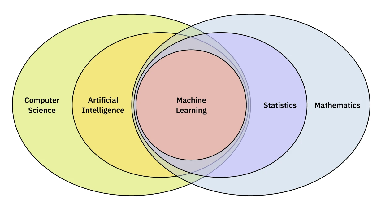
Machine learning is often framed as a subfield of AI, but it stands on its own: a fast-evolving toolkit and practice with no single ‘right’ approach. Recent advances in machine learning have been driven by the development of deep learning, which at least started as a subfield of machine learning that uses deep neural networks to learn from data.

The course is taught as a dialog between Dr. Michael Littman and Dr. Charles Isbell. It opens with a foundational discussion on the philosophy of machine learning. It’s not simply “computational statistics,” as Dr. Littman argues. Instead, Dr. Isbell proposes a broader definition:

This perspective—that machine learning is an interdisciplinary effort to create systems that genuinely learn—shapes the entire curriculum. The goal isn’t just to use algorithms, but to understand them, to “think about data,” and to “build artifacts that you know will learn.”

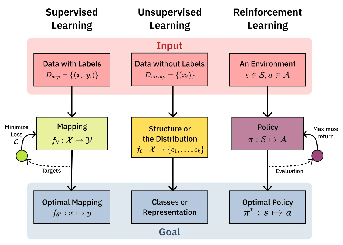
Three core pillars of machine learning make up the foundation of the course: supervised learning, unsupervised learning, and reinforcement learning. Each of these pillars is a different way of learning from data. The most common and well-understood is Supervised learning which involves learning from labeled data. Unsupervised learning is a way to learn from data without labels, and Reinforcement learning is a way to learn from data by interacting with an environment.

This taxonomy provides our roadmap for exploration:

We’ll look at each pillar in turn—starting with supervised learning and its key algorithms, then stepping back for theoretical foundations, before exploring unsupervised learning tools and reinforcement learning. We’ll formalize the mathematical notation as we dive into supervised learning, where these concepts become most concrete.

Mathematical Framing

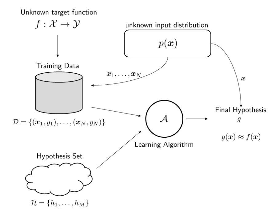
Math is the language of machine learning. Feel free to gloss over it if it’s off putting, there’s still value in building intuition. Defining a few key terms helps to enrich the discussion:

• Data point ($x$): The individual instances of data we want to make predictions about. An instance is typically represented as a vector of features or attributes. The data points are typically a finite sample drawn i.i.d. from some unknown distribution $P(x)$ over the inputs space $\mathcal{X}$ of all possible values of $x$.
• Labels ($y$): The correct answers we want to predict. A label is typically a single value, like a color (“red,” “blue,” “green”) or a simple “yes” or “no.” The output space $\mathcal{Y}$ is the set of all possible values of $y$ and $P(y)$ is the distribution of the labels. The big distinction between supervised and unsupervised learning is whether the labels are provided or not.
• Sample (or Training Set) ($\mathcal{D}$): This is the data we learn from. It’s a set of instances that the learning algorithm uses to find a function within the hypothesis class that best fits the data.
• Concept ($f$): A concept is the function we are trying to learn. It’s a mapping from input instances to outputs. Intuitively, a concept is the underlying idea we want our model to grasp.
  • In supervised learning the classic formulation is $f: \mathcal{X} \rightarrow \mathcal{Y}$, the idea of learning a ‘concept’ from a ‘hypothesis class’.
  • In unsupervised learning, the concept is not a mapping to pre-defined labels, but a function that reveals underlying structure, like a clustering assignment ($f: \mathcal{X} \rightarrow \{c_1, ..., c_k\}$) or a lower-dimensional projection.
  • In reinforcement learning, the core concept being learned is a policy ($\pi$), which is a function mapping states to actions ($\pi: S \rightarrow A$) to maximize long-term reward.

• Target Concept ($f^*$): This is the true, ideal function that we aim to approximate. It’s the perfect, ground-truth mapping that we will never truly know but strive to find.
• Hypothesis Class ($H$): This is the set of all possible concepts our learning algorithm is allowed to consider. By choosing a type of model (like decision trees or neural networks), we are implicitly defining our hypothesis class.
• Candidate Concept: This is a concept from the hypothesis class that our algorithm believes might be the target concept. The learning process involves evaluating different candidate concepts.
• Testing Set: This is a separate set of labeled instances, unseen during training, that we use to evaluate our final candidate concept. A model’s performance on the testing set indicates its ability to generalize to new, unseen data, which is the ultimate goal of machine learning. The training and testing sets must be distinct to avoid “cheating.”

Supervised Learning

Supervised learning is a cornerstone of machine learning. The goal is to learn from labeled data.

With these terms in mind, the process is to use a learning algorithm to search through the hypothesis class ($H$) using the training set to find a final candidate concept that is a good approximation of the target concept ($f^*$), as measured by its performance on the testing set.

The supervised learning hypothesis classes we will explore are:

• Decision Trees: Greedy, interpretable, axis-aligned splits.
• Neural Networks: Layered nonlinear function approximators.
• Ensemble Methods: Combine weak learners to reduce variance and bias.
• Instance-based Learning: Memory-based prediction via similarity (e.g., k-NN).
• Kernel Methods & Support Vector Machines: Max-margin classifiers with kernelized similarity.

Classification and Regression

The two main types of concepts $f$ that can be learned with supervised learning are classification and regression. The key distinction is the nature of the output.

• Classification aims to predict a discrete class label. The output is a category, like a color (“red,” “blue,” “green”) or a simple “yes” or “no.” The learned function is a decision boundary that separates the classes. For example, a bank might use a classification model to decide whether to lend money based on a person’s credit history. The output is a discrete choice: lend or not. We evaluate classification models with metrics like accuracy, precision, recall, and F1-score.
• Regression aims to predict a continuous numerical value. The output is a real number, like a stock price, temperature, or a person’s age. The learned function is a curve or line that best fits the data points. We evaluate regression models with metrics like Mean Squared Error (MSE) or R-squared.

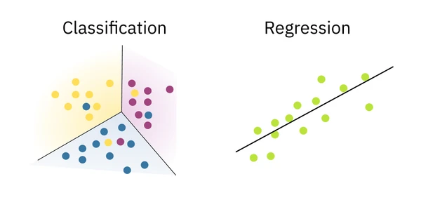
The fundamental difference lies in the output: classification models produce unordered, categorical outputs, while regression models produce ordered, continuous outputs. This distinction guides the choice of algorithms, loss functions, and evaluation metrics. A problem like predicting a person’s age could be framed as either. If you predict their exact age (e.g., 23.7 years), it’s regression. If you predict an age group (e.g., “high school,” “college,” “grad student”), it’s a classification task.

For more details on classification and regression take a look at the lectures Classification and Regression.

Decision Trees

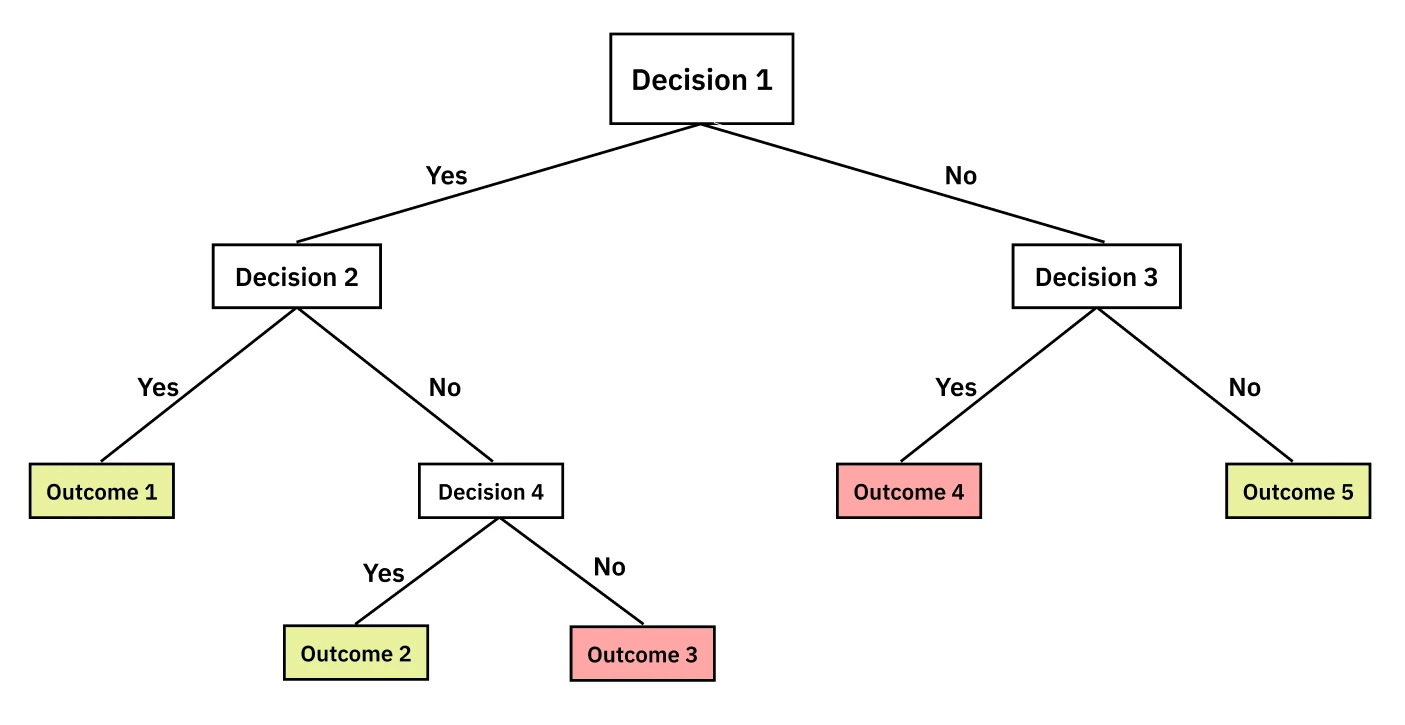
A Decision Tree is a non-parametric supervised learning method that approximates a target function with a tree-like model of decisions. It’s an intuitive model, much like a game of 20 Questions. Each internal node in the tree represents a question about a feature, and the branches represent the answers, leading you down a path to a final decision at a leaf node.

The most common algorithm for building decision trees is ID3, which follows a simple, greedy, top-down approach. It’s best understood through the “20 Questions” analogy: at each step, you want to ask the question that gives you the most information, splitting the remaining possibilities as cleanly as possible.

The ID3 loop is as follows:

1. Select the “best” attribute to split the data on.
2. Create a new decision node for that attribute.
3. For each possible value of the attribute, create a new branch.
4. Sort the training examples down to the new branches.
5. If a branch contains perfectly classified examples, you’re done for that path and can add a leaf node. Otherwise, you repeat the process on the remaining examples in that branch.

The tree structure visually captures this recursive splitting process:

The “best” attribute is the one that provides the highest Information Gain. This metric measures how much a given attribute reduces uncertainty, or entropy, in the data. Entropy is a measure of randomness or impurity—think of it as how “mixed up” the classes are. A dataset with an even split of class labels (e.g., 50% “yes,” 50% “no”) has high entropy, while a dataset with only one class label (e.g., 100% “yes”) has zero entropy. Information gain selects the attribute that leads to the “purest” child nodes—the splits that do the best job of separating the data by their class labels.

ID3 aims to maximize the reduction in entropy at each step, effectively asking the most informative questions first. We’ll revisit entropy with its formal mathematical foundation in the Information Theory section.

20 Questions Example

When playing 20 Questions, you want to ask the question that gives you the most information. For example, if you are trying to guess a person’s name, you might ask if the first letter comes before or after “M”. This is a binary question, and it gives you the most information because it splits the remaining possibilities in half.

This example also illustrates how decision trees can handle continuous attributes. The algorithm might ask a binary question like “Is age < 25.5?”. The optimal split point is typically found by sorting all the values of the continuous attribute in the training data and testing the midpoint between each consecutive pair. This allows you to repeat an attribute along a path (e.g., first ask “Is age < 25.5?” then later “Is age < 20?”) because each split represents a new, distinct question.

Inductive Bias and Overfitting in Decision Trees

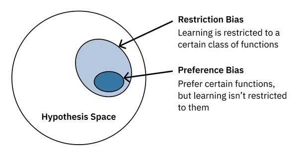
Every type of model (hypothesis class) has a different inductive bias. This is the set of assumptions the model makes about the data. Inductive bias can be thought of as the model’s “prior” knowledge about the data. It comes from the model’s design and structure.

Preference bias is the model’s tendency to favor certain types of solutions (hypotheses) over others within the chosen hypothesis space. Restriction bias is the model’s tendency to favor solutions that are consistent with the data, limiting the set of possible hypotheses that the algorithm can even consider. Both are forms of inductive bias. As we’ll see, every algorithm we explore—from neural networks to ensemble methods—has its own unique inductive biases that shape what it can learn.

For example, decision trees assume that the data is split into a tree-like structure. This is a form of restriction bias. The greedy nature of ID3 gives it a specific preference bias for:

1. Good splits at the top: It will always choose the split that maximizes information gain at the current node.
2. Shorter trees: As a consequence of the first point, it naturally prefers simpler explanations that classify the data quickly. This is a form of Occam’s Razor.

However, this greedy approach can lead to overfitting. The tree might grow very large to perfectly classify every training example, including noisy data. Such a tree would fail to generalize to new, unseen data. To combat this, a common technique is pruning, where parts of the tree are removed post-training to improve its ability to generalize. Another approach is to set a stopping criterion, such as a maximum tree depth or a minimum number of samples required at a leaf node.

Decision trees excel at interpretable, axis-aligned splits but struggle with functions that trees represent inefficiently—like XOR, which requires an exponential number of nodes. This brings us to neural networks, which can learn non-linear functions that decision trees find challenging. For more details checkout the lecture on Decision Trees.

Neural Networks

Artificial Neural Networks (ANNs) are models loosely inspired by the structure of the human brain, but as the course amusingly puts it, they are more of a “cartoonish version of the neuron.” The fundamental building block is the perceptron, a simple computational unit that takes several inputs, multiplies them by weights, sums them up, and fires (outputs a 1) if the sum exceeds a certain threshold, otherwise it outputs a 0.

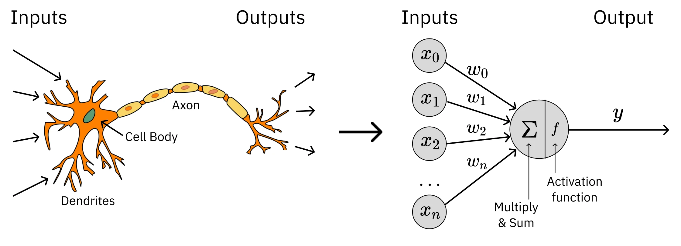
Modern neural networks build on this idea but replace the simple, sharp threshold of the perceptron with a smooth, differentiable activation function like the Sigmoid, Tanh, or ReLU.

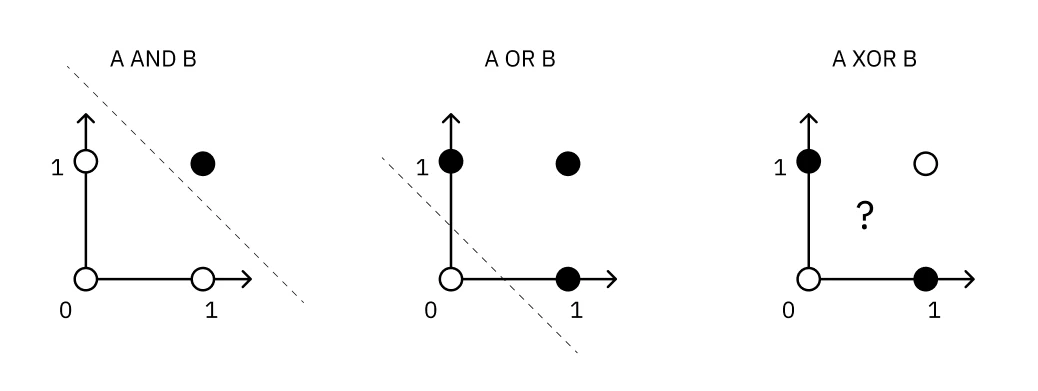
The shift from a hard threshold to differentiable activations is underpinned by the idea of linear separability. A single perceptron can act as a linear separator; for a 2D input space, it can draw a single straight line to divide the space into two halves. This is powerful enough to represent simple logical functions like AND, OR, and NOT, which are all linearly separable. However, a single perceptron fundamentally cannot solve problems that are not linearly separable. The classic example is the XOR function—there is no single straight line you can draw to separate the true cases from the false cases.

This diagram illustrates the key limitation that drives the need for networks of perceptrons:

This limitation is what gives rise to the “network” in neural networks. To solve a problem like XOR, you need to combine perceptrons. For instance, you could use one layer of perceptrons to learn simpler functions (like AND and OR) and then feed their outputs into a final perceptron that combines them to produce the final, non-linear result. This layered structure allows ANNs to learn increasingly complex functions.

Why the switch? The “pointy” nature of the threshold function isn’t differentiable, which is a problem for training. A smooth function allows us to use calculus. The network “learns” by adjusting its weights to minimize a loss function, which measures the difference between the network’s predictions and the actual labels in the training data. The most common training algorithm is backpropagation. At its heart, backpropagation is a clever application of the chain rule from calculus. It uses gradient descent to efficiently compute the contribution of each weight to the overall error and adjust it accordingly. This process is often visualized as error information “flowing” backward from the output layer through the hidden layers, hence the name.

This training process also reveals the biases of neural networks. Recall from Decision Trees that every algorithm has inductive biases—the assumptions it makes about the data. Neural networks have a very different bias profile:

• Restriction Bias: How much does the model’s structure limit the functions it can represent? For ANNs, the restriction bias is very low. With enough layers and nodes, a neural network can approximate any continuous function (and with two hidden layers, any arbitrary function). This makes them universal approximators but also puts them at high risk of overfitting—modeling the noise in the training data instead of the underlying pattern.
• Preference Bias: What kinds of solutions does the learning algorithm prefer? The algorithm itself provides a bias. Training typically starts with small, random weights. As the network trains via gradient descent, it gradually explores more complex functions. This means the algorithm has a preference for simpler explanations, only adopting more complexity as the data requires it. This is a form of Occam’s Razor—we return to a formal justification for this principle later in the Bayesian Learning section. Techniques like early stopping (using a validation set to stop training before the model overfits) explicitly leverage this property.

The power of neural networks lies in this combination of a highly expressive representation (low restriction bias) with a training process that prefers simpler solutions (a helpful preference bias).

For more details, see the Neural Networks lecture which covers:

• How to manually set weights and thresholds for a single perceptron to compute logical functions like AND, OR, and NOT.
• The step-by-step construction of a two-layer network that can solve the non-linearly separable XOR problem.
• The Perceptron Training Rule for single units and its guarantee of convergence for linearly separable data.
• The distinction between the Perceptron Rule (using thresholded outputs) and the Delta Rule / Gradient Descent (using unthresholded activation).
• The common trick of using a “bias input” to allow the learning algorithm to learn the threshold as just another weight.
• The problem of getting stuck in local optima during training and advanced optimization techniques to mitigate it, such as momentum.

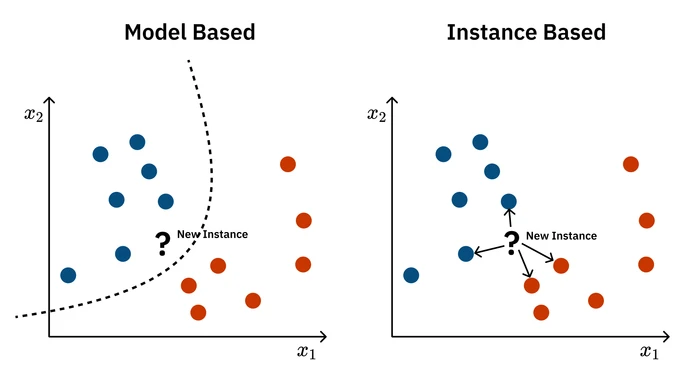
While neural networks offer powerful function approximation through learned representations, they require significant computation for training and can be complex to interpret. Instance-based learning takes a fundamentally different approach: rather than learning an explicit model, why not simply remember all the training examples and make predictions based on similarity?

Instance-based Learning

Instance-based Learning is a fundamentally different approach to machine learning that flips the typical paradigm on its head. Most models we’ve discussed so far are eager learners: they take the training data, learn a generalized function or model, and then effectively throw the original data away. When a new query comes in, they use this compact model to make a prediction. Instance-based learners, in contrast, are lazy learners. They do almost no work upfront, simply storing the entire training dataset. The real computation happens at query time.

This approach is best understood through its most famous algorithm: k-Nearest Neighbors (k-NN). Imagine you’re trying to predict a house price. Instead of building a complex regression model for the whole city, you just find the ‘k’ most similar houses (the “neighbors”) to the one you’re interested in and see what they sold for.

The algorithm is beautifully simple:

1. Store all the training data.
2. When you get a new query point, calculate the distance from that point to every single point in the training data.
3. Identify the ‘k’ nearest neighbors.
4. Aggregate their outputs. For classification, this means taking a majority vote among the neighbors’ classes. For regression, it means averaging their values.

This simplicity is deceptive, as the real “learning” is encoded in two key design choices that represent crucial domain knowledge:

• The distance metric: How do you define “similarity”? For points on a map, Euclidean distance might work. But what about other features? Are all features equally important? A good distance function is critical and is a way to inject domain knowledge into the model. Using a standard metric like Euclidean or Manhattan distance implicitly assumes all features matter equally, which is rarely true.
• The value of k: How many neighbors should you consider? A small ‘k’ makes the model sensitive to noise (an outlier could become a nearest neighbor). A large ‘k’ smooths things out but can be computationally expensive and may blur the lines between distinct regions in your data.

The biggest challenge for k-NN, and a foundational problem in machine learning, is the Curse of Dimensionality. As you add more features (dimensions) to your data, the volume of the space grows exponentially. To maintain the same density of data points, you need an exponentially larger dataset. In a high-dimensional space, the concept of a “neighborhood” breaks down—every point is far away from every other point. Irrelevant features can easily drown out the signal from the important ones, making the distance metric less meaningful.

For more details, see the Instance-Based Learning lecture which covers:

• A comparison of time and space complexity for “lazy” learners (like k-NN) vs. “eager” learners (like linear regression).
• The idea of using distance-weighted averaging or voting to give closer neighbors more influence.
• An example of how different distance metrics (Euclidean vs. Manhattan) can produce wildly different results for the same query.
• How k-NN’s bias towards locality and smoothness means it can perform poorly when features have different levels of importance.
• The concept of locally weighted regression, where instead of just averaging neighbors, you fit a model (like a line) to them, allowing a simple local model to represent a complex global function.

While instance-based learning leverages similarity between data points, individual models often have limitations and biases. What if we could combine multiple models to overcome their individual weaknesses? This leads us to ensemble methods, which harness the collective wisdom of multiple algorithms.

Ensemble Learning

Ensemble learning is a powerful technique that works by combining multiple individual models—often simple “rules of thumb”—to produce a more accurate and robust prediction than any single model could. The lecture uses the great example of classifying spam email. You could have a simple rule like “the email contains the word ‘manly’”, and another like “the email is very short”. Neither is very accurate on its own, but by combining a large set of these weak indicators, you can build a highly effective classifier.

The power of this approach is that the final combined hypothesis can be much more complex and expressive than any of the individual weak learners. By taking a weighted combination of many simple models (like shallow decision trees), the ensemble can form a sophisticated, non-linear decision boundary that it couldn’t have represented otherwise. It’s a way of getting a complex result from simple parts.

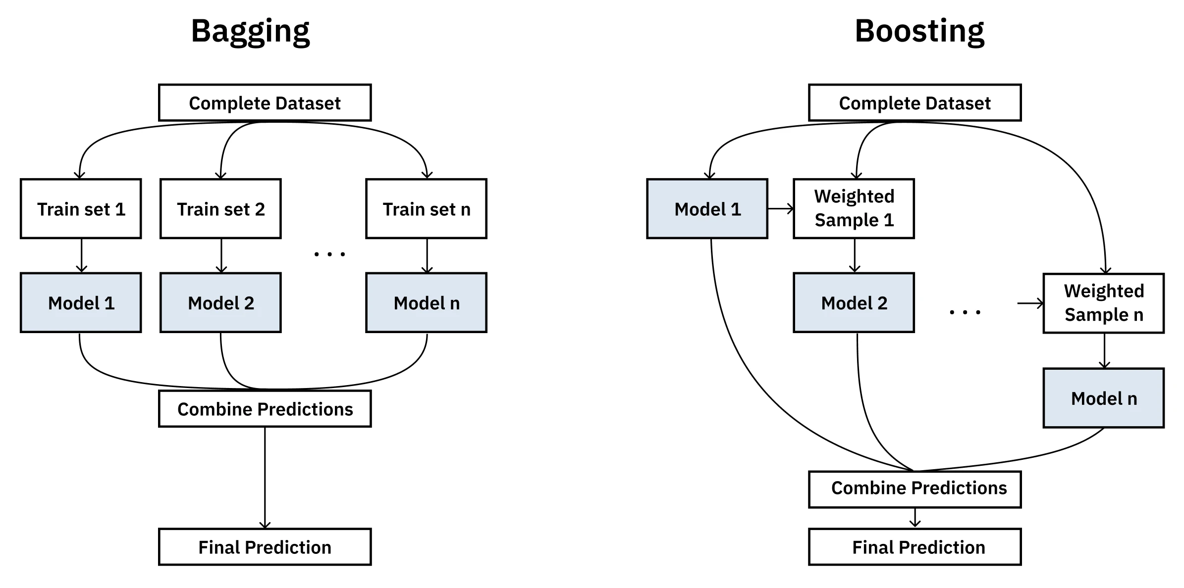
The two primary families of ensemble methods, Bagging and Boosting, are different approaches to this same core idea.

• Bagging (Bootstrap Aggregating): This method follows a simple and surprisingly effective process. It involves training multiple instances of the same model (e.g., decision trees) on different random subsets of the training data. The subsets are created by bootstrapping, which means sampling with replacement. The final prediction is made by averaging the outputs of all models (for regression) or by taking a majority vote (for classification). Random Forests are a popular and effective implementation of this approach. The main benefit of bagging is that it reduces variance and helps prevent overfitting. By averaging out the “opinions” of models trained on different views of the data, it’s less likely to be swayed by noise.

• Boosting: This method takes a more strategic approach. Instead of training on random subsets, boosting builds models sequentially, where each new model is explicitly tasked with correcting the errors made by the previous ones. The algorithm maintains a distribution of “weights” over the training examples. In each round, it trains a weak learner—an algorithm that only needs to be slightly better than random chance—on the weighted data. After each round, it increases the weights of the examples that were misclassified, forcing the next weak learner to focus on the “hard” cases. The final model is a weighted combination of all the weak learners, where models that performed better on their respective rounds are given a greater say in the final prediction. Popular boosting algorithms include AdaBoost and Gradient Boosting Machines (GBMs).

Perhaps the most remarkable property of boosting is its surprising resistance to overfitting. With most algorithms, as we continue to train, the model gets better and better on the training data, but at some point, the performance on unseen test data starts to get worse—the classic sign of overfitting. Boosting often defies this. In practice, even as the training error goes to zero, the test error can continue to improve as more weak learners are added. While the full explanation is complex, the intuition is that even after the model correctly classifies all training points, adding more weak learners can increase the margin of the classification, making the decision boundary more robust and improving generalization.

For more details, see the Ensemble Learning lecture which covers:

• The formal definition of a “weak learner” as a classifier that can always perform slightly better than chance (error < 0.5) on any distribution of data.
• A visual walkthrough of how boosting combines simple axis-aligned classifiers to create a complex, non-linear decision boundary.
• The specific formulas used in the AdaBoost algorithm to update the data distribution and calculate the alpha weights for each weak learner.

Ensemble methods show how combining simple models can create sophisticated decision boundaries. But what if we want a single, elegant model that can also handle complex, non-linear relationships? Support Vector Machines achieve this through a different approach: finding the optimal separating boundary and using mathematical tricks to handle non-linearity.

Kernel Methods & Support Vector Machines

Support Vector Machines (SVMs) are a powerful and versatile class of supervised learning models. The lecture explains them beautifully, starting with a simple question: if you have two groups of points that can be separated by a straight line, what is the best line?

The answer isn’t just any line that separates the data. The best line is the one that shows the “least commitment” to the training data, giving us the best chance to generalize to new data. This line is the one that creates the widest possible “demilitarized zone” or street between the two classes. This zone is called the margin, and the goal of an SVM is to find the separating hyperplane that maximizes this margin. The data points that lie on the very edge of this margin—the ones that “support” the hyperplane—are called the support vectors. If you move any other point, the line doesn’t change. But if you move a support vector, the optimal line will move with it.

This visualization shows how SVMs balance between fitting the data and maximizing generalization:

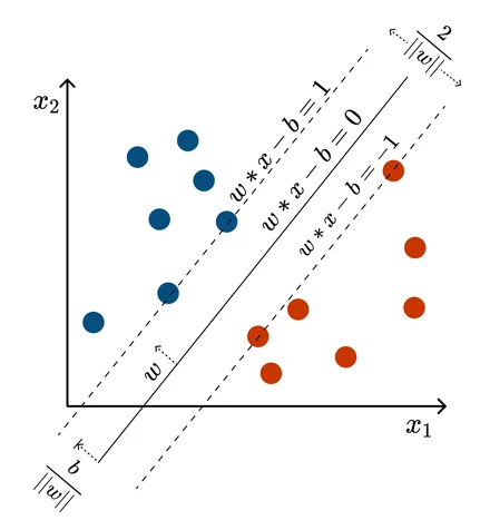
This intuition can be formalized into an optimization problem. The goal is to maximize the margin, which turns out to be equivalent to minimizing the squared norm of the weight vector ($1/2 ||w||^2$), subject to the constraint that every data point is correctly classified and lies outside the margin. This constraint for each point $i$ is captured by the elegant expression: $y_i(w^T x_i + b) \ge 1$. This is a well-defined quadratic programming problem that can be solved efficiently.

But what happens when the data isn’t linearly separable? Imagine a cluster of positive points surrounded by a ring of negative points. No straight line can separate them. This is where one of the most powerful ideas in machine learning comes into play: the kernel trick.

The idea is to project the data into a higher-dimensional space where it becomes linearly separable. For the ring example, we could map our 2D data into a 3D space, lifting the points in the center up higher than the points in the ring, allowing us to slice a plane between them. The magic of the kernel trick is that we can achieve this without ever actually paying the computational cost of creating these higher-dimensional representations.

This geometric transformation illustrates the elegance of the kernel approach:

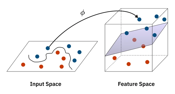
Instead of transforming the data, we modify our optimization algorithm. The algorithm only ever needs to compute the dot product between pairs of data points ($x_i^T x_j$) to measure their similarity. The kernel trick involves replacing this simple dot product with a more complex kernel function, $K(x_i, x_j)$. For example, using the kernel $K(x_i, x_j) = (x_i^T x_j)^2$ is mathematically equivalent to mapping the data into a higher-dimensional space and computing the dot product there, but it’s vastly more efficient.

The kernel function is essentially a pluggable measure of similarity. This allows us to inject domain knowledge into the model. Common kernels include:

• Linear: The standard dot product, for data that is already linearly separable.
• Polynomial: $K(x,y) = (x^T y + c)^p$. Captures polynomial relationships in the data.
• Radial Basis Function (RBF): $K(x,y) = \exp(-\gamma ||x-y||^2)$. A very popular and flexible kernel that can handle complex, non-linear relationships. It’s a good default choice.

By using the kernel trick, SVMs can learn highly complex, non-linear decision boundaries, making them effective for a wide range of problems.

For more details, see the Kernel Methods & SVMs lecture which covers:

• The derivation of maximizing the margin as an optimization problem.
• The dual formulation of the SVM problem, which explicitly introduces the kernel function.
• How support vectors are the data points with non-zero alpha values in the dual solution.
• How kernels can be defined over non-vector data like strings and graphs.

We’ve now explored a diverse toolkit of supervised learning algorithms—from interpretable decision trees to powerful neural networks to elegant support vector machines. But a crucial question remains: why do these algorithms work? Before we shift to unsupervised learning and reinforcement learning, let’s ground what we’ve seen in formal learning theory to understand the fundamental principles that govern when and why learning is possible.

What to remember

• Key takeaways before moving on:

• Classification vs. regression: discrete labels vs. continuous values drive algorithm, loss, and metrics choices.

• Hypothesis classes: trees (interpretable), neural nets (expressive), ensembles (variance/bias reduction), instance-based (similarity), SVMs (max-margin + kernels).

• Overfitting control: pruning/early stopping, validation, and margins help generalization.

• Kernel trick: compute similarity via kernels to model non-linear boundaries efficiently.

• Generalization: always evaluate on held-out data; test performance is the goal.

Theoretical Foundations of Learning

These theoretical frameworks help explain why and when learning is possible, providing rigorous foundations for the algorithms we’ve explored and the principles that guide effective machine learning.

Computational Learning Theory

Computational Learning Theory (CoLT) provides the formal tools to answer fundamental questions about learning. It’s not just about building models that work; it’s about understanding why they work and when we can be confident in their predictions. The theory helps us define what a learning problem is, show that certain algorithms can solve it, and even prove that some problems are fundamentally hard.

The key resource in machine learning is data. CoLT helps us quantify how much data we need to learn effectively. This is called sample complexity. The goal is to learn a concept that is Probably Approximately Correct (PAC). This framing acknowledges two realities:

1. Approximately Correct: We can’t expect our learned model to be perfect. There will always be some error. The goal is to ensure the true error (the error on the underlying data distribution) is less than some small value, $\epsilon$ (pronounced “epsilon”).
2. Probably: We can never be 100% certain. There’s always a chance we got a misleading set of training examples. The goal is to be at least $1 - \delta$ (pronounced “delta”) confident that our learned model has an error less than $\epsilon$.

A key concept for understanding PAC learning is the version space. The version space is the set of all hypotheses in our hypothesis class that are consistent with the training data. The learning process is essentially a search for a good hypothesis within this space.

Making It Concrete: What Do $\epsilon$ and $\delta$ Actually Mean?

Before diving into the mathematical bounds, let’s make these parameters concrete. Imagine you’re building a spam email classifier:

• $\epsilon$ (error tolerance): You might set $\epsilon = 0.05$, meaning you want your classifier to have at most 5% error on new emails. This is your accuracy requirement.
• $\delta$ (confidence): You might set $\delta = 0.1$, meaning you want to be 90% confident (1 - 0.1 = 0.9) that your classifier will indeed achieve this 5% error bound. This accounts for the possibility that you got unlucky with your training data.

The question CoLT answers is: How many training emails do you need to achieve 5% error with 90% confidence?

Sample Complexity Bounds

A central result from CoLT, Haussler’s Theorem, gives us a concrete bound on the number of samples ($m$) needed to guarantee PAC-learnability for a finite hypothesis space ($H$):

$$m \ge \frac{1}{\epsilon} \left( \ln|H| + \ln\frac{1}{\delta} \right)$$

Example: Let’s return to our spam classifier. Suppose you’re using a simple decision tree that can ask 10 binary questions about an email (e.g., “Does it contain ‘FREE!’?”, “Is the sender address suspicious?”). Your hypothesis space has at most $2^{2^{10}} \approx 10^{308}$ possible trees. With $\epsilon = 0.05$ and $\delta = 0.1$:

$$\begin{aligned} m &\ge \frac{1}{0.05} \left( \ln(10^{308}) + \ln(10) \right) \\ &\approx 20 \left( 708.4 + 2.3 \right) \\ &\approx 14,214 \text{ training emails} \end{aligned}$$

This calculation shows you need at least 14,214 training examples to be 90% confident your classifier will have at most 5% error on new emails.

This is a powerful result. It tells us that the number of examples we need only grows linearly with $1/\epsilon$ and logarithmically with the size of our hypothesis space and $1/\delta$. However, it raises a critical question: what happens when our hypothesis space is infinite, as is the case for linear separators, neural networks, or decision trees with continuous features?

VC Dimension

The Vapnik-Chervonenkis (VC) Dimension is the answer to that question. It’s a way to measure the “effective” size or “expressive power” of a hypothesis class, even if it’s infinite. The VC dimension is defined as the size of the largest set of points that the hypothesis class can shatter.

To “shatter” a set of points means the hypothesis class can generate every possible labeling for those points.

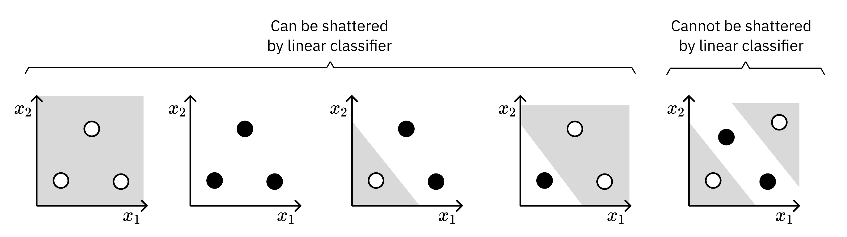
For example, a linear separator in a 2D plane has a VC dimension of 3. You can arrange three points in a triangle, and a line can achieve all 8 possible +/- labelings. However, there is no arrangement of four points that a single line can shatter. Specifically, if you arrange four points in a way that forms a convex hull and assign alternating labels (like an XOR pattern), no single line can separate them—this is precisely the limitation that drove us to neural networks when we discussed the XOR problem.

VC Dimension and Sample Complexity

The insight of VC dimension is that it provides a finite measure of complexity even for infinite hypothesis classes. The VC dimension cleverly replaces the $\ln|H|$ term in our sample complexity bound, giving us a practical way to compute how much data we need:

$$m \ge \frac{1}{\epsilon} \left( 8 \cdot \text{VC}(H) \log_2\frac{13}{\epsilon} + 4 \log_2\frac{2}{\delta} \right)$$

Example: Consider using a linear classifier for our spam detection problem. Since we’re working with, say, 100 email features (word counts, sender patterns, etc.), our linear separator in 100D space has VC dimension = 101. Using the same $\epsilon = 0.05$ and $\delta = 0.1$:

$$\begin{aligned} m &\ge \frac{1}{0.05} \left( 8 \cdot 101 \cdot \log_2\frac{13}{0.05} + 4 \cdot \log_2\frac{2}{0.1} \right) \\ &\approx 20 \left( 808 \cdot 8.02 + 4 \cdot 4.32 \right) \\ &\approx 129,940 \text{ emails} \end{aligned}$$

Interestingly, this requires far more data than our finite decision tree example! This illustrates an important principle: higher VC dimension means greater model complexity, which requires more data to learn reliably.

This theorem is profound. It tells us that as long as a hypothesis class has a finite VC dimension, it is PAC-learnable, regardless of whether it contains an infinite number of hypotheses. The VC dimension captures the true complexity of the model, and a finite VC dimension prevents the model from being too powerful and overfitting the data. It’s the key that connects the expressive power of a model to its ability to generalize from a finite sample of data.

For more details, see the Computational Learning Theory and VC Dimension lectures, which cover:

• Different models of learning based on how training examples are selected (learner queries vs. helpful teacher vs. nature).
• The mistake bound model of learning.
• The concept of epsilon-exhausting the version space.
• How to prove the VC dimension for different hypothesis classes like intervals and polygons.
• The relationship between VC dimension and the number of parameters in a model.

VC dimension tells us when learning is possible by measuring model complexity. But it doesn’t tell us how to choose between competing hypotheses that all fit the data. This brings us to Bayesian learning, which provides a principled framework for reasoning about uncertainty and choosing the most probable hypothesis.

Bayesian Learning + Inference

Bayesian learning offers a probabilistic view on machine learning, framing it as a quest to find the most probable hypothesis given our data. This shifts the perspective from finding a single “best” model to reasoning about a whole distribution of possible models. The foundation for this is the elegant Bayes’ Theorem.

Here’s how it breaks down in a machine learning context:

• $P(h|D)$ (Posterior): What we want to find. The probability of a hypothesis $h$ being correct after seeing the data $D$.
• $P(D|h)$ (Likelihood): How well the hypothesis $h$ explains the data. It’s the probability of observing data $D$ if $h$ were true. This is often easier to calculate.
• $P(h)$ (Prior): Our prior belief about the hypothesis $h$ before seeing any data. This is where we can inject domain knowledge, such as a preference for simpler models.
• $P(D)$ (Evidence): The probability of the data. This term is a normalization constant and is often ignored when comparing hypotheses, as it doesn’t depend on $h$.

The core idea is to start with a prior belief ($P(h)$) and update it as we collect evidence ($D$), resulting in a more informed posterior belief ($P(h|D)$).

Priors Matter: An Intuitive Example

The power of the prior is beautifully illustrated by a classic example. Imagine a highly accurate test for a very rare disease. The test is 98% accurate for positive results and 97% for negative. The disease is incredibly rare, occurring in only 0.8% of the population.

A patient tests positive. Do they have the disease?

Surprisingly, no. The probability that they don’t have the disease is much higher. The extremely low prior probability of having the disease outweighs the test’s accuracy. The tiny chance of a false positive is more likely than the tiny chance of actually having the disease. This demonstrates that our initial beliefs (priors) are a critical component of our reasoning.

From Probabilities to Practical Algorithms

The Bayesian framework provides a theoretical foundation for many well-known machine learning concepts.

MAP and Maximum Likelihood

Our goal is to find the Maximum a Posteriori (MAP) hypothesis—the one that maximizes $P(h|D)$. This is equivalent to maximizing $P(D|h)P(h)$.

If we don’t have any prior beliefs and assume all hypotheses are equally likely (a uniform prior), the $P(h)$ term becomes a constant. Our task then simplifies to finding the Maximum Likelihood (ML) hypothesis, which just maximizes the likelihood $P(D|h)$.

Connection to Sum of Squared Errors

One of the most profound results from this framework is the justification for using sum of squared errors. If we assume that our data is generated by a deterministic function but corrupted by Gaussian (normal distribution) noise, then finding the Maximum Likelihood hypothesis is mathematically equivalent to minimizing the sum of squared errors between our model’s predictions and the actual data.

This means that whenever you use linear regression or train a neural network by minimizing mean squared error, you are implicitly making an assumption of Gaussian noise in your data!

Connection to Occam’s Razor

Bayesian learning also provides a formal justification for Occam’s Razor—the principle that simpler explanations are better. This is done through the Minimum Description Length (MDL) principle.

By applying some information theory, finding the MAP hypothesis can be shown to be equivalent to finding the hypothesis that minimizes the sum of two things:

1. The “length” or complexity of the hypothesis itself (e.g., the number of nodes in a decision tree).
2. The “length” of the description of the data’s errors, given the hypothesis.

This creates a natural trade-off: a more complex model might reduce the error, but it pays a penalty for its own complexity. The best model is the one that finds the sweet spot, providing the most compact explanation for the data.

The Real Goal: Bayesian Classification

So far, we’ve focused on finding the single best hypothesis. But what if the goal is to make the most accurate prediction on a new data point?

The most likely hypothesis (the MAP hypothesis) might not always give the most likely prediction. The lecture gives a great example:

• h1 predicts + with probability 0.4
• h2 predicts - with probability 0.3
• h3 predicts - with probability 0.3

The MAP hypothesis is h1, which predicts +. However, the total probability for the label - is 0.3 + 0.3 = 0.6. The most probable label is actually -.

This leads to the Bayes Optimal Classifier. Instead of picking one hypothesis and discarding the others, we let every hypothesis “vote” on the final prediction, with their vote weighted by their posterior probability. On average, no other classifier can perform better. It provides a theoretical gold standard for classification.

This is a powerful idea: finding the best model is just a means to an end. The ultimate goal is to make the best predictions.

For more detail, see the lectures on Bayesian Learning and Bayesian Inference. The lectures also cover:

• The connection to Version Spaces, where in noise-free settings, all consistent hypotheses are equally probable.
• Detailed mathematical derivations for the Sum of Squared Error (from Gaussian noise) and Minimum Description Length (from information theory).
• The concept of a Joint Probability Distribution and the curse of dimensionality.
• Bayesian Networks (Belief Networks) as a graphical way to represent conditional independencies.
• Exact and approximate inference techniques for querying Bayesian Networks.
• The Naive Bayes Classifier, including its strong (“naive”) independence assumption and its practical effectiveness.
• The need for smoothing (like Laplace smoothing) to handle zero-frequency problems in Naive Bayes.

With these theoretical foundations in place—understanding when learning is possible, how much data we need, and how to reason about uncertainty—we can now turn to the second pillar of machine learning: learning from data without labels.

What to remember

• PAC learning: target small error (ε) with high confidence (1-δ); sample complexity scales with model complexity.
• VC dimension: capacity measure that replaces ln|H| for infinite hypothesis classes.
• Bayesian view: combine priors and likelihoods (MAP/ML); MDL formalizes Occam; SSE arises from Gaussian noise.
• Information theory: entropy and mutual information justify splits and feature scoring.
• Big picture: explains when learning is possible, how much data you need, and how to choose among hypotheses.

Unsupervised Learning

Unlike supervised learning, which relies on labeled data to learn a mapping from inputs to outputs, unsupervised learning ventures into the messier, more common world of unlabeled data. The goal shifts from prediction to discovery. Instead of approximating a known function, the aim is to perform “data description”—to find the inherent structure, patterns, and more compact representations hidden within the data itself. This makes it less of a single, crisply-defined problem and more a diverse set of tools for understanding data, including the topics we’ll explore next: randomized optimization, clustering, and feature transformation.

Randomized Optimization

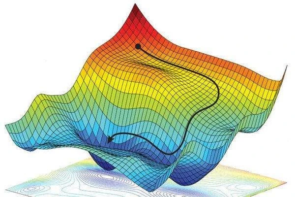
Randomized optimization algorithms are a class of methods used to find good approximate solutions to complex optimization problems, especially when the search space is vast or the objective function is “unfriendly”—meaning it’s not smooth, continuous, or easily differentiable. The core idea is to introduce randomness into the search process to escape local optima and explore the solution space more effectively. As the lecture puts it, they are essential when you can’t just use calculus to find the peak. They are often used in machine learning to tune the weights of a neural network, as an alternative to backpropagation—recall from our Neural Networks discussion how gradient descent can get stuck in local optima.

• Randomized Hill Climbing (RHC): This is the simplest algorithm, akin to a mountain climber in a thick fog who can only feel the ground immediately around them. It starts with a random solution and at each step, generates a random neighbor. If the neighbor is higher up the “hill” (i.e., has a better fitness score), the climber moves there. This process continues until no better neighbor can be found. The main drawback is that it can easily get stuck on a small hill (a local optimum), missing the highest peak (the global optimum). A common enhancement is random-restart hill climbing, where if the climber gets stuck, they are helicoptered to a new random spot on the mountain to start climbing again.
• Simulated Annealing (SA): SA improves on hill climbing by giving the climber the ability to occasionally take a step downhill. This helps it escape local optima and cross valleys to find bigger hills. The probability of accepting a worse solution is controlled by a “temperature” parameter. Initially, the temperature is high, and the climber is very energetic, willing to jump around and explore wildly. As the temperature gradually “cools,” the climber becomes less likely to take downward steps, eventually settling into a final, hopefully optimal, position. This process is inspired by the metallurgical process of annealing, where a blacksmith heats and slowly cools a sword to allow its molecules to settle into a strong, low-energy crystal structure.

• Genetic Algorithms (GAs): Inspired by the process of natural selection, GAs work with a whole population of climbers scattered across the mountain. At each “generation,” the “fittest” climbers (those with the best solutions) are selected to “reproduce.” They combine their “genes” (features of their solutions) through an operation called crossover, creating new “offspring” solutions. To maintain diversity, small random changes (mutation) are also introduced. This creates a new generation of solutions, and the process is repeated. GAs are highly effective at exploring large and complex search spaces by sharing information between parallel searches.

• MIMIC (Mutual-Information-Maximizing Input Clustering): MIMIC is a more “amnesiac” algorithm that, unlike its predecessors, tries to learn from its experience. Instead of just keeping track of the best points found so far, MIMIC builds a probabilistic model of the promising regions of the search space. It explicitly estimates the probability distribution of good solutions, and then samples new points from this model to generate the next generation. By modeling the structure of the good parts of the space, it can often find the optimum in far fewer iterations, which is a huge advantage when evaluating the fitness function is expensive (e.g., running a complex simulation or requiring human feedback).

For more details, see the Randomized Optimization lecture, which covers:

• The fundamental trade-off between exploration (searching the space) and exploitation (using local information to improve).
• How to define a neighborhood function for problems like guessing a bit string.
• The concept of a basin of attraction and how its size affects the performance of random-restart hill climbing.
• The Boltzmann distribution and its role in the probabilistic acceptance of moves in Simulated Annealing.
• Different types of crossover operators in Genetic Algorithms, such as one-point and uniform crossover.
• How MIMIC turns the optimization problem into a problem of finding a maximum spanning tree to model feature dependencies.

Randomized optimization helps us find good solutions when the search space is complex. But sometimes we need to understand the data itself rather than optimize a function. This brings us to clustering, which seeks to discover the natural groupings hidden within our data.

Clustering

Clustering is a fundamental task in unsupervised learning where the goal is to group a set of objects in such a way that objects in the same group (or cluster) are more similar to each other than to those in other groups. Unlike supervised learning, there are no predefined labels. The algorithm must discover the inherent structure in the data on its own.

The lecture emphasizes that clustering isn’t one single, well-defined problem; it’s a family of algorithms, each with its own notion of what a “good” cluster is. The choice of algorithm and its parameters (like the number of clusters, ‘k’) is a way to inject crucial domain knowledge into the process.

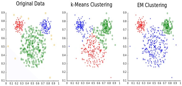
• Single-Linkage Clustering (SLC): This is a type of hierarchical agglomerative clustering (HAC). It’s a “bottom-up” approach that starts by treating each data point as its own cluster. Then, it iteratively merges the two closest clusters until a stopping condition is met. The “single-linkage” part defines the distance between two clusters as the distance between their closest two points. This can lead to long, “stringy” clusters, as the algorithm can create chains of points, which may not always match our intuitive sense of a compact cluster.
• k-Means Clustering: This is one of the most popular and intuitive clustering algorithms. It aims to partition the data into ‘k’ clusters by iteratively assigning each data point to the cluster with the nearest mean (or centroid) and then recalculating the centroids based on the new assignments. This process is a form of optimization; it’s a hill-climbing algorithm that is guaranteed to converge by minimizing the sum of squared distances from each point to its assigned centroid. However, it can get stuck in local optima, so the initial random placement of centroids matters.
• Expectation-Maximization (EM): EM provides a more probabilistic approach to clustering, often used with Gaussian Mixture Models (GMMs). Instead of making a “hard” assignment of each point to a single cluster, EM performs soft clustering. It calculates the probability that each data point belongs to each cluster. It’s a two-step process: the E-step (Expectation) calculates these probabilities, and the M-step (Maximization) updates the parameters of the clusters (like their means and variances) to maximize the likelihood of the data given these assignments. This allows for more flexible, elliptically-shaped clusters and provides a measure of uncertainty in the assignments, which is a key advantage over the hard assignments of k-Means.

A fascinating result from the theory of clustering is Kleinberg’s Impossibility Theorem. It proves that no clustering algorithm can simultaneously satisfy three very desirable properties: richness (can produce any possible clustering), scale-invariance (result doesn’t change if you switch from miles to kilometers), and consistency (shrinking distances within clusters and expanding them between clusters doesn’t change the result). This highlights that there is no single “best” clustering algorithm, and the choice always involves trade-offs.

For more details, see the Clustering lecture which covers:

• Different ways to define the distance between clusters in hierarchical clustering, such as average-linkage and complete-linkage.
• The connection between single-linkage clustering and finding a minimum spanning tree.
• A proof of why the k-Means algorithm is guaranteed to converge.
• The use of hidden variables in the Expectation-Maximization (EM) algorithm.
• How EM can be seen as a “soft” version of k-Means.

Clustering groups data points by similarity, but what if our data has too many dimensions or contains irrelevant noise? This is where feature selection and transformation become essential—helping us identify and work with the most meaningful aspects of our data.

Feature Selection

Feature selection is the process of selecting a subset of relevant features (variables, predictors) for use in model construction. The goal is to improve model performance by removing irrelevant or redundant features, which can reduce overfitting, improve accuracy, and reduce training time.

There are three main types of feature selection methods:

• Filter Methods: These methods rank features based on some statistical score (like correlation or mutual information with the target variable) and then select the top-ranked features. They are fast and independent of the chosen learning algorithm.
• Wrapper Methods: These methods use a specific machine learning algorithm to evaluate the quality of different subsets of features. They search for the combination of features that results in the best model performance, but they can be computationally expensive.
• Embedded Methods: These methods perform feature selection as part of the model training process itself. A classic example is L1 regularization (Lasso), which adds a penalty to the model’s loss function based on the absolute value of the feature weights, effectively shrinking the weights of less important features to zero.

For more details on feature selection, see the lecture on Feature Selection.

Feature selection chooses which existing features to keep, but sometimes we need to go further and create entirely new features that better capture the underlying patterns. This is where feature transformation techniques like PCA and ICA become powerful tools for dimensionality reduction and representation learning.

Feature Transformation

Feature transformation, or dimensionality reduction, is the process of transforming data from a high-dimensional space into a lower-dimensional space, while preserving some meaningful properties of the original data. This can help to visualize the data, reduce computational complexity, and remove noise. Feature selection can be seen as a specific type of feature transformation where the transformation is simply selecting a subset of the original features.

The lecture uses the example of information retrieval to illustrate the need for feature transformation. If you’re searching for “car,” you also want documents that use the word “automobile” (synonymy), but you don’t want documents about Lisp programming just because it uses a car function (polysemy). Simple feature selection (picking which words to use) can’t solve this. Feature transformation addresses this by creating new, combined features from the original ones.

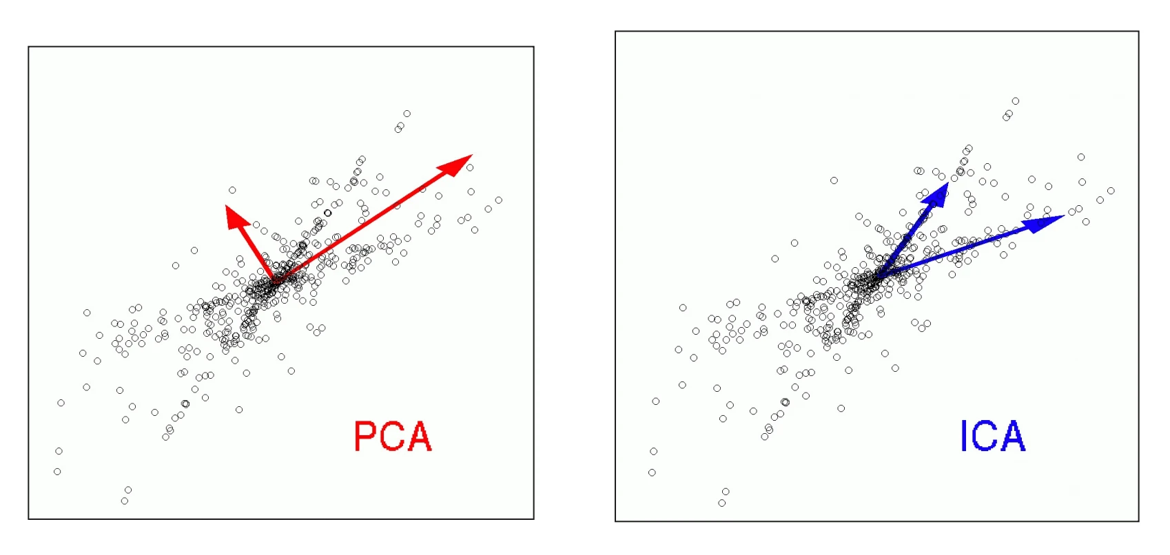
• Principal Component Analysis (PCA): PCA is a linear technique that finds a new set of orthogonal axes, called principal components, that capture the maximum amount of variance in the data. The data is then projected onto a smaller number of these components. It’s a powerful tool for dimensionality reduction because it provides the best possible reconstruction of the original data from a lower-dimensional projection, minimizing the L2 error. However, the directions of maximum variance may not always be the most useful for a classification task.
• Independent Component Analysis (ICA): ICA is another linear technique that, instead of maximizing variance, seeks to find a transformation where the new features are statistically independent. The classic example is the “cocktail party problem,” where ICA can take mixed audio signals from multiple microphones and separate them back into the original, independent sources (e.g., individual voices). When applied to images, ICA tends to find “parts” like edges and noses, whereas PCA finds more global features like the “average face.”
• Random Component Analysis (RCA): This method, also known as random projection, simply projects the data onto a random set of lower-dimensional vectors. Surprisingly, it works remarkably well. While it doesn’t offer the same guarantees as PCA for reconstruction, it’s extremely fast and can be very effective for classification tasks, as it still manages to preserve some of the correlational structure of the original data. It’s a great example of a simple, “cheap” method that often provides a strong baseline.
• Linear Discriminant Analysis (LDA): Unlike the previous methods, LDA is a supervised dimensionality reduction technique. It explicitly uses the class labels to find a projection that maximizes the separability between the classes. This makes it a “wrapper” method in spirit, as it’s concerned with how the features will be used for a downstream classification task, not just with the inherent structure of the data itself.

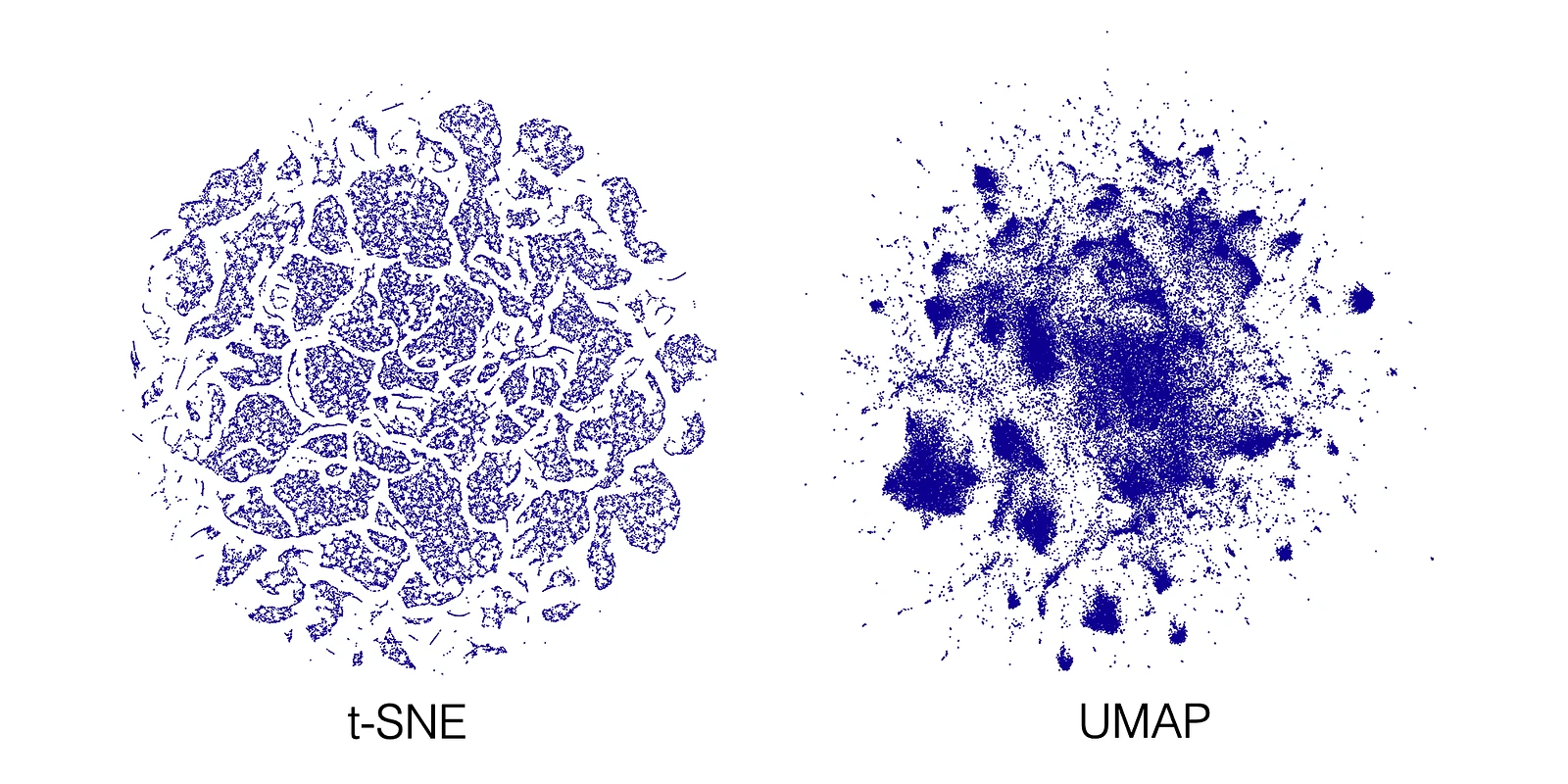
• t-SNE (t-Distributed Stochastic Neighbor Embedding): t-SNE is a non-linear technique that is particularly well-suited for visualizing high-dimensional datasets. It models each high-dimensional object by a two- or three-dimensional point in such a way that similar objects are modeled by nearby points and dissimilar objects are modeled by distant points with high probability.
• UMAP (Uniform Manifold Approximation and Projection): UMAP is another non-linear technique for manifold learning and dimensionality reduction. It is often faster than t-SNE and can better preserve the global structure of the data.

For more details, see the lecture on Feature Transformation, which covers:

• The distinction between feature transformation as a linear algebra problem (PCA) vs. a probability/information theory problem (ICA).
• How PCA finds directions of maximal variance that are mutually orthogonal.
• How ICA, by assuming non-Gaussian sources, can separate mixed signals where PCA cannot.
• The surprising effectiveness of Random Component Analysis (RCA) as a fast and simple baseline.

Information Theory

Information theory is a mathematical framework for quantifying information, originally developed by Claude Shannon at Bell Labs to solve a very practical problem: how to charge for sending a message. The key insight was that a message’s value isn’t its length, but the amount of “surprise” or uncertainty it resolves.

In our discussion of Decision Trees, we introduced the concepts of entropy and information gain as intuitive tools for selecting the best attribute at each split. Information theory provides the formal mathematical foundation for these ideas.

Recall from Decision Trees that entropy measures how “mixed up” or impure a dataset is. Now we can formalize this: entropy $H$ measures the average number of bits required to represent an event from a probability distribution, calculated as:

$$H(X) = -\sum_{i=1}^{n} p_i \log_2(p_i)$$

Where

• $H(X)$ is the entropy of the attribute $X$.
• $n$ is the number of classes in the attribute $X$.
• $p_i$ is the probability of the $i$th class in the attribute $X$.
• $\log_2$ is the base-2 logarithm, reflecting the bits of information needed to specify the outcome. The base-2 is used because we split between two choices (e.g. binary, yes/no) at each node.

A fair coin flip has an entropy of 1 bit, while a biased coin has entropy closer to 0. This concept is the heart of variable-length encoding, like Morse code, where more frequent letters (like ‘E’ and ‘T’) are given shorter codes to make messages more efficient.

Building on this foundation, we can define other key concepts that are critical in machine learning:

• Conditional Entropy ($H(Y|X)$): Measures the remaining uncertainty about variable Y after you know variable X. For example, the uncertainty about whether you’ll hear thunder ($Y$) is much lower if you already know it’s raining ($X$).
• Mutual Information ($I(X;Y)$): This measures the reduction in uncertainty about Y that comes from knowing X. This should sound familiar: the Information Gain we used in our ID3 algorithm is precisely the Mutual Information between a feature and the class label. It quantifies how much a feature tells us about the final classification.
• Kullback-Leibler (KL) Divergence: Measures the difference, or “distance,” between two probability distributions. It’s often used as a loss function in machine learning to measure how well a model’s predicted distribution matches the true distribution of the data.

For more details, see the lecture on Information Theory.

What to remember

• Key takeaways before moving on:

• Randomized optimization: explore search spaces when gradients fail (RHC, SA, GA, MIMIC).

• Clustering: different objectives (SLC, k-Means, EM); no single best method (Kleinberg’s theorem).

• Feature selection vs. transformation: choose relevant features vs. create new representations (PCA/ICA/RCA/LDA).

• Visualization vs. structure: t-SNE/UMAP for visualization; PCA/ICA for structure and compression.

• Information theory: entropy, mutual information, and KL underpin feature selection and splitting criteria.

Reinforcement Learning

The course then transitions to Reinforcement Learning (RL), the third major paradigm of machine learning. Unlike supervised or unsupervised learning, RL is concerned with how an agent can learn to make a sequence of decisions in an environment to maximize a cumulative reward. This section follows the course’s structure, starting with the mathematical framework for decision-making, Markov Decision Processes (MDPs). It then delves into core RL algorithms that solve these problems when the environment’s dynamics are unknown. Finally, it extends these concepts to scenarios with multiple agents using the principles of Game Theory.

Markov Decision Processes (MDPs)

A Markov Decision Process (MDP) is a mathematical framework for modeling decision-making in situations where outcomes are partly random and partly under the control of a decision-maker. It is the formal foundation for reinforcement learning. The lecture introduces this concept using an intuitive Grid World example: imagine an agent on a grid, trying to reach a goal with a positive reward (+1) while avoiding a pitfall with a negative reward (-1).

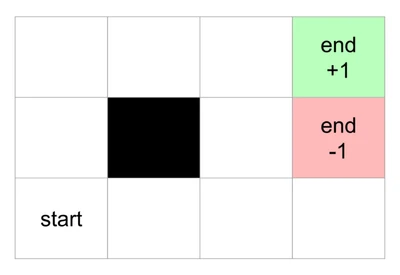
An MDP is defined by a few key components:

• A set of states ($S$): The agent’s possible locations on the grid.
• A set of actions ($A$): The moves the agent can make (e.g., up, down, left, right).
• A transition model $T(s, a, s')$: The probability of transitioning from state $s$ to state $s'$ after taking action $a$. This is where uncertainty comes in. An action might not always succeed; for example, trying to move “up” might only work 80% of the time, with a 10% chance of moving left and a 10% chance of moving right instead.
• A reward function $R(s, a, s')$: The immediate reward received after a transition. In the grid world, this is mostly a small negative value (e.g., -0.04) for each step, encouraging efficiency, with a large positive or negative reward at the terminal states.

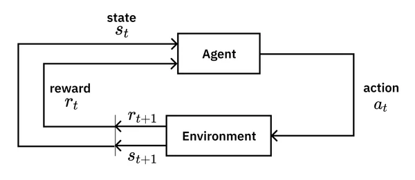
The agent’s behavior is governed by a policy $\pi(s)$, which is a mapping from states to actions. Recall from our initial definitions that a policy ($\pi: S \rightarrow A$) is the core concept learned in reinforcement learning. Unlike a fixed plan (e.g., “up, up, right, right”), a policy tells the agent what to do in any state it finds itself in, making it robust to the stochastic nature of the world.

The core assumption of an MDP is the Markov Property: the next state and reward depend only on the current state and action, not on the entire history of how the agent got there.

The goal in an MDP is to find an optimal policy $\pi^*(s)$ that maximizes the long-term cumulative expected reward. Simply summing rewards can be problematic in worlds with infinite horizons, as the total reward could be infinite. To solve this, we introduce a discount factor $\gamma$ (a value between 0 and 1), which makes future rewards less valuable than immediate ones. The total utility of a state sequence becomes a discounted sum: $U = \sum_{t=0}^{\infty} \gamma^t R(s_t)$.

The Bellman Equation is the cornerstone for solving MDPs. It defines the utility of a state recursively in terms of the utilities of its neighboring states: $U(s) = R(s) + \gamma \max_{a \in A} \sum_{s' \in S} T(s, a, s') U(s')$

This equation tells us that the utility of a state is the immediate reward plus the discounted expected utility of the best action from that state. We can find the optimal utilities, and thus the optimal policy, using algorithms like Value Iteration or Policy Iteration.

For more details, see the Markov Decision Processes lecture which covers:

• The distinction between plans and policies in deterministic vs. stochastic environments.
• The difference between immediate rewards and long-term utility.
• The concepts of finite vs. infinite time horizons and how they affect the optimal policy.
• The derivation of the discounted rewards formula as a geometric series.
• A detailed walkthrough of the Value Iteration and Policy Iteration algorithms.
• How to turn a non-Markovian problem into a Markovian one by expanding the state definition.

Reinforcement Learning Lecture

The last section laid out the planning problem: if we know the complete model of the world—the transition probabilities $T(s, a, s')$ and the reward function $R(s, a, s')$—we can use algorithms like Value Iteration to find an optimal policy. But what happens when we don’t have a model?

This is where Reinforcement Learning (RL) comes in. RL tackles the more realistic scenario where an agent must learn to act in an environment without prior knowledge of its dynamics. The problem is no longer one of planning with a known model, but of learning from direct experience.

Instead of being given a model, an RL agent learns from experience, which comes in the form of transitions: a set of tuples (s, a, r, s'), representing the agent being in state s, taking action a, receiving reward r, and ending up in state s'.

There are three main approaches to RL:

• Model-based RL: First, learn the transition and reward models from experience. Then, use planning algorithms (like Value Iteration) to find the optimal policy.
• Value Function-based RL: Directly learn a value function that estimates the long-term reward. The policy is then derived from this value function.
• Policy Search: Directly search for the optimal policy without explicitly learning a value function or a model.

A key concept in value-based RL is the Q-function (or state-action value function), denoted $Q(s, a)$. It represents the value of taking action $a$ in state $s$ and then following the optimal policy thereafter. The Bellman equation for the Q-function is: $Q(s, a) = R(s) + \gamma \sum_{s' \in S} T(s, a, s') \max_{a' \in A} Q(s', a')$ With the Q-function, the optimal policy is simple: in any state $s$, choose the action $a$ that maximizes $Q(s, a)$.

Q-learning is a model-free, value-based algorithm that directly learns the optimal Q-function from transitions. It uses the following update rule: $Q(s, a) \leftarrow Q(s, a) + \alpha \left( r + \gamma \max_{a'} Q(s', a') - Q(s, a) \right)$

Here, $\alpha$ is the learning rate. This update moves the current Q-value for $(s, a)$ a little bit closer to the temporal difference (TD) target ($r + \gamma \max_{a'} Q(s', a')$), which is a better estimate of the true value based on the reward received and the estimated value of the next state.

A fundamental challenge in RL is the exploration-exploitation dilemma: the agent must decide whether to exploit its current knowledge to get high rewards or to explore new actions to potentially discover even better rewards. A common strategy is epsilon-greedy, where the agent chooses the best-known action most of the time but explores a random action with a small probability $\epsilon$.

For more details, see the Reinforcement Learning lecture which covers:

• The API of reinforcement learning and its components (modeler, simulator, planner, learner).
• A brief history of the term “reinforcement learning” from psychology.
• The concept of “optimism in the face of uncertainty” as an exploration strategy.
• How TD Gammon, a famous backgammon-playing program, used a simulator and a learner.
• The conditions for Q-learning convergence (Greedy in the Limit with Infinite Exploration - GLIE).

So far we’ve focused on single agents learning in isolation. But what happens when multiple intelligent agents interact in the same environment, each pursuing their own goals? This is where game theory provides the mathematical framework for understanding strategic interaction and multi-agent learning.

Game Theory

Game theory is the study of mathematical models of strategic interaction among rational decision-makers. In machine learning, it provides a powerful framework for understanding multi-agent systems, where multiple agents interact within the same environment. The lectures introduce game theory as the “mathematics of conflict,” a natural extension of reinforcement learning from a single agent to multiple agents.

Key concepts include:

• Players: The decision-makers in the game.
• Strategies: The possible actions each player can take. A pure strategy is a deterministic choice, while a mixed strategy is a probability distribution over choices.
• Payoffs: The outcomes or rewards for each player, often represented in a payoff matrix.

A fundamental distinction is made between different types of games:

• Zero-Sum vs. Non-Zero-Sum: In zero-sum games, one player’s gain is another’s loss. In non-zero-sum games, players can have outcomes that are mutually beneficial or mutually harmful.
• Perfect vs. Hidden Information: In games of perfect information, all players know the state of the game at all times. With hidden information, players may not know what cards the others hold, as in poker.

Minimax and Nash Equilibrium

For two-player, zero-sum games with perfect information, the Minimax algorithm provides a solution. Each player assumes the other will make the move that is best for them and worst for the opponent. The goal is to maximize one’s own minimum possible payoff.

However, in more complex, non-zero-sum games, a more general solution concept is needed: the Nash Equilibrium. A set of strategies is a Nash Equilibrium if no player can do better by unilaterally changing their strategy.

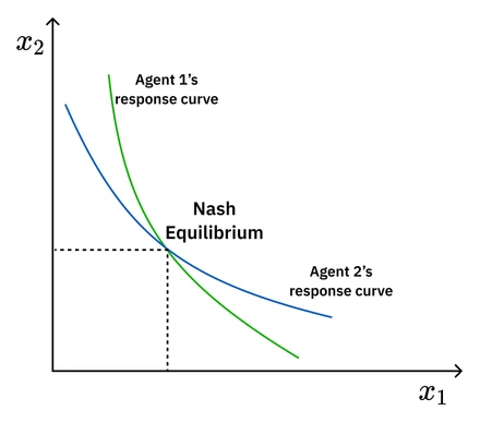
Repeated Games and Cooperation

The dynamics of game theory change significantly when games are repeated over time. The Iterated Prisoner’s Dilemma shows that if the number of rounds is known, players will always defect. However, if the end is uncertain (modeled with a discount factor, $\gamma$), cooperation can emerge.

This leads to the Folk Theorem, which states that in a repeated game, any feasible payoff profile that is better for all players than the worst-case (minmax) payoff can be a Nash Equilibrium. This is achieved through strategies that reward cooperation and punish defection. A famous example is Tit-for-Tat, where a player starts by cooperating and then copies the opponent’s previous move. This simple strategy promotes long-term cooperation.

By modeling multi-agent problems as games, we can analyze the dynamics of competition and cooperation and design agents that can learn to behave strategically in the presence of other intelligent agents.

For more details, see the lectures on Game Theory I and Game Theory II, which cover:

• The different types of games (zero-sum, non-zero-sum, deterministic, non-deterministic, perfect/hidden information).
• The distinction between pure and mixed strategies.
• The concept of a “security level profile” and how it’s calculated.
• The Folk Theorem and its implications for achieving cooperation in repeated games.
• Strategies for repeated games like Grim Trigger, Tit-for-Tat, and Pavlov.
• The idea of subgame perfect equilibrium and plausible threats.
• Stochastic (or Markov) games as a generalization of MDPs for multi-agent reinforcement learning.
• Reinforcement learning algorithms for multi-agent settings, such as Minimax-Q and Nash-Q.

What to remember

• Key takeaways before moving on:

• MDP anatomy: states, actions, transitions, rewards, discount; policies map states to actions.

• Bellman equation: recursive definition of value enables planning (value/policy iteration).

• Q-learning: model-free update toward TD target; derive policy from learned Q.

• Exploration: epsilon-greedy and optimism trade off exploration vs. exploitation.

• Game theory: beyond single-agent—Nash equilibrium, repeated games, cooperation dynamics.

Course Overview

The course was taught with a huge focus on the projects. These emphasized the conceptual material presented in the lectures through hands-on research and experimentation. They were a great way to solidify the concepts learned in the course and took up a significant portion of the time I spent on the course.

Here are the projects from the course:

• Project 1: Supervised Learning
• Project 2: Randomized Optimization
• Project 3: Unsupervised Learning & Dimensionality Reduction
• Project 4: Reinforcement Learning

Grading

Here’s the grading breakdown from when I took the course in Fall 2024. There was a pretty generous curve at the end of the semester.

Component	Weight	Mean	Q1	Median	Q3	High
Hypothesis Quiz	5%	78.60%	70.00%	80.00%	90.00%	100.00%
Reading Quiz	5%	97.04%	100.00%	100.00%	100.00%	100.00%
Project 1	15%	68.13%	56.00%	73.00%	85.00%	105.00%
Project 2	15%	69.26%	60.00%	73.00%	83.00%	100.00%
Project 3	15%	72.95%	65.00%	79.00%	87.00%	105.00%
Project 4	15%	75.83%	71.00%	81.00%	91.00%	105.00%
Final	30%	67.77%	60.91%	70.93%	78.89%	102.42%

Books

These are some classic books in Machine Learning that complement the course material.

Other Resources

Here are some other posts I found helpful:

• Monzer Saleh’s notes
• George Kudrayvtsev’s notes
• Swyx’s posts that cover most of the lectures
• Yi Xiang’s overview of the experience of taking the course
• Eugene Yan’s Review and Tips

My Experience

I took ML alongside High Performance Computer Architecture and stayed disciplined—starting projects as soon as they were released. That made the workload manageable despite the course’s breadth and open-ended nature. I enjoyed—and was also wary of—how easy it is to go deep on any of these topics. This survey was just an introduction to a rich, fascinating field. I’ve continued to dig in!

---

Thanks for reading!

References